What is Gradient Descent? The Ultimate Guide to the Algorithm that Powers Machine Learning

If you’ve ever wondered how machine learning models “learn” from data to make accurate predictions, you’ve stumbled upon the most critical concept behind the magic: Gradient Descent.

It’s not an exaggeration to call Gradient Descent the backbone of modern machine learning. From the simplest linear regression to the most complex deep neural networks, this optimization algorithm is the workhorse that tunes models to perfection.

But what exactly is it? How does it work? And why is it so fundamental?

In this comprehensive guide, we will demystify Gradient Descent. We’ll start with a simple analogy, dive into the core mechanics, explore its different variants, and address common challenges. By the end, you’ll have a thorough understanding of the algorithm that enables AI to learn.

read more about Cross-Validation in Machine Learning: The Definitive Guide to Building Robust Models

A Simple Analogy: The Blindfolded Hiker

Imagine you’re a hiker on a large, foggy hill, blindfolded. Your goal is to find the lowest point in the valley. You can’t see the entire landscape, but you can feel the steepness of the ground beneath your feet.

What would you do?

You would take a small step in the direction where the ground descends most steeply. You’d feel again and take another step down. You’d repeat this process—feeling the slope and taking steps downward—until the ground beneath you feels flat. At that point, you’ve (hopefully) reached the lowest point in the valley.

This is the essence of Gradient Descent.

• You, the hiker: The machine learning model.
• The Hilly Landscape: The cost (or loss) function—a mathematical function that measures how wrong the model’s predictions are. A higher point means a bigger error.
• The Lowest Valley: The minimum of the cost function, where the model’s predictions are as accurate as possible.
• Feeling the Steepness: Calculating the gradient. In mathematics, the gradient is a vector that points in the direction of the steepest ascent of a function. Gradient Descent uses the negative of the gradient, which points downhill.
• Taking a Step: Updating the model’s parameters (like weights and biases) with a small adjustment. The size of this step is the learning rate.

The Formal Definition of Gradient Descent

Gradient Descent is an iterative, first-order optimization algorithm used to find a local minimum of a differentiable function.

Let’s break down that definition:

• Iterative: It works by repeating the same process over and over.
• First-Order: It uses the first derivative (the gradient) of the function, not second-order derivatives.
• Optimization Algorithm: Its purpose is to minimize (or maximize) a function.
• Differentiable: The function must have a derivative at every point we want to evaluate it.

In machine learning, that function is almost always the Cost Function (J(θ)). The parameters we are trying to optimize are the model’s weights (θ). The goal is to find the parameters θ that minimize J(θ).

The Core Gradient Descent Algorithm: A Step-by-Step Breakdown

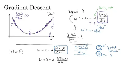
The algorithm can be summarized in a single, powerful update rule:

θ = θ - η * ∇J(θ)

Don’t be intimidated by the math. Let’s dissect it piece by piece:

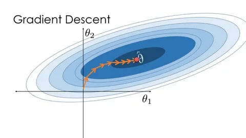
1. Initialize: Start by guessing the initial values for the model’s parameters (θ). This is like randomly placing the blindfolded hiker on the hill.
2. Iterate until convergence: Repeat the following steps:
   • Calculate the Gradient (∇J(θ)): Compute the gradient of the cost function with respect to each parameter. This tells us the direction and magnitude of the steepest ascent.
   • Take a Step in the Opposite Direction: Since we want to go downhill, we take the negative of the gradient.
   • Update the Parameters: Multiply the gradient by the Learning Rate (η – “eta”) and subtract this from the current parameters. The formula θ = θ - η * ∇J(θ) updates all parameters simultaneously.

This process repeats until the algorithm converges, meaning the parameters no longer change significantly and the cost function has (hopefully) reached a minimum.

The Heart of the Algorithm: The Learning Rate (η)

The learning rate is the most critical hyperparameter in Gradient Descent. It determines the size of the steps we take towards the minimum.

The choice of learning rate has a profound impact:

• Learning Rate is Too Small:
  • Consequence: Very slow convergence.Analogy: The hiker takes tiny, timid steps. It will take a very long time to reach the bottom, and they might get stuck in a very small dip (a local minimum) early on.
• Learning Rate is Too Large:
  • Consequence: Divergence. The algorithm overshoots the minimum and fails to find a solution, often leading to an increase in the cost function.Analogy: The hiker takes massive leaps, potentially jumping from one side of the valley to the other, completely missing the lowest point.
• Learning Rate is Optimal:
  • Consequence: The algorithm finds the minimum efficiently and reliably.

Finding the right learning rate is often an empirical process and is crucial for training effective models.

The Three Flavors of Gradient Descent

There are three main variants of the algorithm, which differ in how much data they use to compute the gradient.

1. Batch Gradient Descent

• How it works: Uses the entire training dataset to compute the gradient of the cost function for one update.
• Pros:
  • Computationally efficient for small datasets.
  • Provides a stable path to the minimum and guaranteed convergence.
• Cons:
  • Can be extremely slow for very large datasets since it must process the entire dataset for a single step.
  • Can get stuck in local minima (as opposed to the global minimum).

2. Stochastic Gradient Descent (SGD)

• How it works: Uses a single training example (a single data point) to compute the gradient for one update.
• Pros:
  • Much, much faster for large datasets.
  • The inherent randomness helps it jump out of local minima, potentially finding a better global minimum.
• Cons:
  • The path to the minimum is very noisy and erratic. It never truly settles at the minimum but oscillates around it.
  • Loses the computational advantages of vectorization.

3. Mini-Batch Gradient Descent

• How it works: This is the goldilocks solution and the most common method used in practice. It uses a small, random subset (a “mini-batch”) of the training data (e.g., 32, 64, or 128 examples) for each update.
• Pros:
  • Compromise between the stability of Batch GD and the speed of SGD.
  • Allows for efficient hardware optimization (especially GPUs).
  • Smoother convergence than SGD.
• Cons:
  • Introduces the mini-batch size as a new hyperparameter to tune.

Type	Data Used Per Step	Speed	Stability	Common Use
Batch	Entire Dataset	Slow	High	Small Datasets
Stochastic (SGD)	Single Example	Fast	Low (Noisy)	Large, Redundant Datasets
Mini-Batch	Small Subset (Mini-batch)	Fast & Efficient	Medium	Default for Deep Learning

Common Challenges and Solutions in Gradient Descent

The path to the optimal model is not always smooth. Here are key challenges and how modern optimization techniques address them.

1. Local Minima vs. Global Minimum

• Problem: The cost function landscape can have many “dips” (local minima), but only one true “lowest point” (global minimum). Standard Gradient Descent can get stuck in a local minimum, thinking it has found the best solution.
• Solution: Stochastic Gradient Descent (SGD). The randomness in its steps helps it bounce out of local minima, making it more likely to find a much better solution.

2. Vanishing/Exploding Gradients

• Problem: Especially in deep neural networks, gradients can become extremely small (vanish) or extremely large (explode) as they are propagated back through the layers. This stops the network from learning effectively.
• Solution: Careful weight initialization strategies (e.g., He or Xavier initialization) and specific activation functions (like ReLU) help mitigate this. More advanced optimizers like Adam are also more robust.

3. Saddle Points

• Problem: A saddle point is a flat region where the gradient is zero but is not a minimum. It’s a point where in some directions the slope goes up, and in others, it goes down. Gradient Descent can get stuck here.
• Solution: Again, the noise in SGD or the momentum in advanced optimizers can help push the algorithm through saddle points.

Beyond Basic Gradient Descent: Advanced Optimizers

While the core concept remains, several advanced algorithms build upon Gradient Descent to improve performance:

• Momentum: Helps accelerate Gradient Descent in the relevant direction and dampens oscillations. It’s like a ball rolling downhill, gaining momentum.
• Adam (Adaptive Moment Estimation): One of the most popular and effective optimizers today. It combines the concepts of Momentum and adaptive learning rates for each parameter.

Conclusion: Why Gradient Descent is Indispensable

Gradient Descent is a remarkably powerful and elegant solution to the fundamental problem of optimization in machine learning. By iteratively moving in the direction that reduces error, it provides a systematic way for models to learn from data and improve their performance.

To recap:

• It’s an iterative optimization algorithm.
• It uses gradients to find the direction of steepest descent.
• The learning rate controls the size of its steps.
• Mini-batch Gradient Descent is the most widely used variant in practice.
• Understanding its challenges, like local minima and the importance of the learning rate, is key to applying it successfully.

Whether you are building a recommendation system, a self-driving car, or a simple predictor, Gradient Descent is likely working under the hood, tirelessly guiding your model toward greater intelligence. It truly is the engine of machine learning.