Linear Regression Explained for Beginners: Theory & Python Code

Linear Regression is the cornerstone of predictive analytics and a fundamental algorithm in Machine Learning. If you’re starting your journey into data science, mastering Linear Regression is your first crucial step. It’s not just a model; it’s a concept that opens the door to understanding more complex algorithms.

This ultimate beginner’s guide will walk you through everything you need to know: from the basic intuition and underlying mathematics to a complete, hands-on Python implementation. By the end of this article, you will have a solid grasp of what Linear Regression is, how it works, and how to build your own predictive model from scratch.

What is Linear Regression? (The Simple Intuition)

At its heart, Linear Regression is a statistical method used to model the relationship between a dependent variable and one or more independent variables. The goal is simple: to predict a value.

Let’s break that down with a classic example:

Imagine you want to predict the price of a house. What factors influence the price?

• Size (sq. ft.)
• Number of Bedrooms
• Age of the House
• Location

In this scenario:

• The House Price is our dependent variable (the ‘target’ we want to predict).
• The Size, Bedrooms, Age, and Location are our independent variables (the ‘features’ we use for prediction).

Linear Regression finds a linear relationship between these features and the target. It essentially draws the “best-fit” straight line (or a hyperplane in higher dimensions) through your data points.

Types of Linear Regression

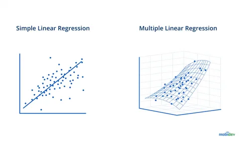
1. Simple Linear Regression: Involves only one independent variable to predict a dependent variable.
   • Formula: y = mx + b
   • Example: Predicting house price based only on its size.
2. Multiple Linear Regression: Involves two or more independent variables to predict a dependent variable.
   • Formula: y = b₀ + b₁x₁ + b₂x₂ + ... + bₙxₙ
   • Example: Predicting house price based on size, bedrooms, age, and location.

The Mathematics Behind Linear Regression: How Does it Find the “Best-Fit” Line?

How does the algorithm determine which line is the “best”? The answer lies in the Ordinary Least Squares (OLS) method.

The core idea is to minimize the error between the predicted values and the actual values.

Key Concepts:

• The Hypothesis Function: This is the equation of our line.
  • For Simple LR: h(x) = θ₀ + θ₁x (where θ₀ is the intercept, θ₁ is the slope)
  • For Multiple LR: h(x) = θ₀ + θ₁x₁ + θ₂x₂ + ... + θₙxₙ
• Cost Function (Mean Squared Error – MSE): This function measures how wrong our predictions are. It’s the average of the squared differences between the actual values (y) and the predicted values (h(x)).
  • MSE = (1/n) * Σ(Actualᵢ - Predictedᵢ)²
  • Where n is the number of data points.
• The Goal: The learning process involves adjusting the parameters (θ₀, θ₁, …, θₙ) to find the values that minimize the MSE. A lower MSE means a better-fitting model.

Gradient Descent is the optimization algorithm often used to find these optimal parameters. It iteratively adjusts the parameters to move “downhill” on the cost function curve until it finds the minimum value. Think of it as walking down a valley until you reach the lowest point.

read more about How to Choose the Right Machine Learning Algorithm

---

Hands-On Tutorial: Implementing Linear Regression in Python

Now for the practical part! We will use Python’s powerful scikit-learn library to build a Multiple Linear Regression model.

Step 1: Importing Necessary Libraries

We’ll start by importing all the essential tools.

python

# For data manipulation and analysis
import pandas as pd
import numpy as np

# For data visualization
import matplotlib.pyplot as plt
import seaborn as sns

# For machine learning models and tools
from sklearn.model_selection import train_test_split
from sklearn.linear_model import LinearRegression
from sklearn.metrics import mean_absolute_error, mean_squared_error, r2_score

# Magic command for Jupyter notebooks to display plots inline
%matplotlib inline

Step 2: Loading and Exploring the Dataset

For this tutorial, we’ll use a simple sample dataset. In practice, you would load your own CSV file.

python

# Create a sample dataset
data = {
    'Size_sqft': [650, 785, 1200, 1400, 1550, 1800, 2100, 2400, 2750, 3000],
    'Bedrooms': [1, 2, 3, 3, 3, 4, 4, 5, 5, 5],
    'Age': [15, 10, 5, 8, 2, 1, 12, 3, 1, 2],
    'Price': [320000, 385000, 550000, 610000, 650000, 720000, 760000, 800000, 890000, 920000]
}

# Create a DataFrame
df = pd.DataFrame(data)

# Display the first 5 rows
print(df.head())

Output:

text

   Size_sqft  Bedrooms  Age   Price
0        650         1   15  320000
1        785         2   10  385000
2       1200         3    5  550000
3       1400         3    8  610000
4       1550         3    2  650000

Step 3: Performing Exploratory Data Analysis (EDA)

Before modeling, it’s crucial to understand the data.

python

# Get a quick statistical summary
print(df.describe())

# Visualize the relationships between features and target
sns.pairplot(df)
plt.show()

# Check the correlation matrix
plt.figure(figsize=(8, 6))
sns.heatmap(df.corr(), annot=True, cmap='coolwarm', linewidths=0.5)
plt.title('Correlation Matrix')
plt.show()

The pairplot and correlation matrix help you see which features have the strongest linear relationship with the price (e.g., Size_sqft is likely highly correlated with Price).

Step 4: Preparing the Data

We need to split our data into features (X) and target (y), and then into training and testing sets.

python

# Define features (X) and target (y)
X = df[['Size_sqft', 'Bedrooms', 'Age']] # Independent variables
y = df['Price'] # Dependent variable

# Split the data: 80% for training, 20% for testing
X_train, X_test, y_train, y_test = train_test_split(X, y, test_size=0.2, random_state=42)

print(f"Training set size: {X_train.shape}")
print(f"Testing set size: {X_test.shape}")

Step 5: Creating and Training the Model

This is where we create our Linear Regression model and “fit” it to our training data.

python

# Create an instance of the LinearRegression model
model = LinearRegression()

# Train the model on the training data
model.fit(X_train, y_train)

The fit method is where the magic happens—the algorithm learns the parameters (θ₀, θ₁, θ₂, θ₃) that minimize the cost function for our data.

Step 6: Making Predictions

Now, let’s use our trained model to make predictions on the test data.

python

# Make predictions on the test set
y_pred = model.predict(X_test)

# Create a DataFrame to compare actual vs predicted values
results = pd.DataFrame({'Actual': y_test, 'Predicted': y_pred})
print(results)

Step 7: Evaluating the Model Performance

How good is our model? We use evaluation metrics to answer this.

python

# Calculate key performance metrics
mae = mean_absolute_error(y_test, y_pred)
mse = mean_squared_error(y_test, y_pred)
rmse = np.sqrt(mse) # Root Mean Squared Error
r2 = r2_score(y_test, y_pred)

print(f"Mean Absolute Error (MAE): ${mae:,.2f}")
print(f"Mean Squared Error (MSE): ${mse:,.2f}")
print(f"Root Mean Squared Error (RMSE): ${rmse:,.2f}")
print(f"R-squared (R²) Score: {r2:.4f}")

Interpreting the Metrics:

• MAE/MSE/RMSE: Measure the average error of the model. Lower values are better. RMSE is especially useful as it is in the same units as the target variable (dollars, in our case).
• R-squared (R²): Represents the proportion of the variance in the dependent variable that is predictable from the independent variables. It ranges from 0 to 1. A higher value (closer to 1) is better. An R² of 0.95 means 95% of the variation in house prices is explained by our model’s features.

Step 8: Understanding the Model Coefficients

Let’s look at the equation our model has created.

python

# Get the intercept and coefficients
print(f"Intercept (θ₀): ${model.intercept_:.2f}")

# Display coefficients alongside their feature names
coefficients = pd.DataFrame(model.coef_, X.columns, columns=['Coefficient'])
print(coefficients)

Interpretation:

• Intercept (θ₀): The predicted price when all features are zero (often not practically meaningful on its own).
• Coefficient for ‘Size_sqft’: For every additional square foot, the price increases by [Coefficient Value] dollars, assuming all other features remain constant.
• Coefficient for ‘Age’: For every additional year in the house’s age, the price decreases by [Coefficient Value] dollars (if the coefficient is negative), assuming all other features remain constant.

This interpretability is a key strength of Linear Regression.

---

Assumptions of Linear Regression

For the model to be reliable, its key assumptions should be met:

1. Linearity: The relationship between features and target is linear.
2. Independence: Observations are independent of each other.
3. Homoscedasticity: The variance of errors is constant across all levels of the independent variables.
4. Normality: The errors of the model are normally distributed.
5. No Multicollinearity: The independent variables are not highly correlated with each other.

Conclusion: Your First Step into Machine Learning

Congratulations! You’ve just built and evaluated your first Linear Regression model. You’ve learned:

• The intuition behind this fundamental algorithm.
• The core mathematics of how it finds the best-fit line.
• How to implement it in Python using scikit-learn from start to finish.
• How to evaluate your model’s performance and interpret its results.

Linear Regression is a powerful and interpretable tool for prediction. While real-world datasets are often more complex, the principles you’ve learned here are universal. This knowledge forms the bedrock for understanding more advanced algorithms like Logistic Regression, Polynomial Regression, and even Neural Networks.

Ready to practice? Find a dataset on Kaggle (like the Boston Housing dataset) and try to build your own regression model. The world of machine learning is now at your fingertips.