How to Evaluate a Machine Learning Model: Accuracy, Precision, Recall & F1 Explained

To effectively evaluate a machine learning model, you must look beyond a single performance score. This guide will show you how to use metrics like accuracy, precision, and recall to get a complete picture of your model’s strengths and weaknesses. Understanding how to evaluate a machine learning model is essential for deploying reliable AI systems.

Why Accuracy Isn’t Enough

Many people start by looking at accuracy, but this is rarely sufficient. Accuracy can be misleading, especially with imbalanced datasets. A true, effective model evaluation digs deeper to understand the types of errors the model makes, which is where precision and recall become critical.

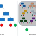
read more about Decision Trees and Random Forests Made Easy: Your Ultimate Guide

What would its accuracy be? 99%.

It sounds fantastic, but it’s utterly useless. It has failed to identify even a single sick person. This is known as the “Accuracy Paradox,” where a high-accuracy model is practically worthless.

To see the full picture, we need a more nuanced tool: the Confusion Matrix.

The Confusion Matrix: The Foundation of All Metrics

The Confusion Matrix is a table that breaks down your model’s predictions into four distinct categories. It’s the bedrock for calculating Precision, Recall, and F1.

Let’s use a binary classification example (e.g., “Spam” vs. “Not Spam”) to define these categories:

	Predicted: SPAM	Predicted: NOT SPAM
Actual: SPAM	True Positive (TP) You correctly identified spam.	False Negative (FN) You missed spam (it went to the inbox).
Actual: NOT SPAM	False Positive (FP) You flagged a good email as spam.	True Negative (TN) You correctly left a good email in the inbox.

• True Positive (TP): The model correctly predicted the positive class.
• False Positive (FP): The model incorrectly predicted the positive class (a “Type I Error”).
• False Negative (FN): The model incorrectly predicted the negative class (a “Type II Error”).
• True Negative (TN): The model correctly predicted the negative class.

This matrix gives you a complete picture of your model’s performance, warts and all. Now, let’s use it to build our key metrics.

Precision: The Measure of Quality

Precision answers the question: “When the model predicts ‘positive,’ how often is it correct?”

It focuses on the quality of the positive predictions. A high-precision model is trustworthy when it flags something.

Precision = TP / (TP + FP)

Think of it as: “How precise are our positive claims?”

When is High Precision Critical?

• Search Engine Results: When you perform a search, you want the top results to be highly relevant (i.e., not junk). False positives are bad.
• Spam Detection: If your model flags an important client’s email as spam (a False Positive), the consequences can be severe. You’d rather let a few spam emails through (False Negatives) than lose a critical email.

Recall: The Measure of Completeness

Recall (or Sensitivity) answers the question: “Of all the actual positives, how many did the model correctly identify?”

It focuses on the model’s ability to find all the relevant cases. A high-recall model leaves very few positives behind.

Recall = TP / (TP + FN)

Think of it as: “How many of the true positives did we recall/catch?”

When is High Recall Critical?

• Disease Screening: In a cancer detection model, you want to catch every single case of cancer. A missed case (a False Negative) could be fatal. It’s acceptable to have a few false alarms (False Positives) if it means finding all the sick patients.
• Fraud Detection: You want to identify as many fraudulent transactions as possible. Letting a fraudster through (False Negative) is far costlier than flagging a legitimate transaction for review (False Positive).

The Tug-of-War: Precision vs. Recall

In an ideal world, we want both perfect Precision and perfect Recall. In reality, they often exist in a trade-off.

• Increasing Precision typically reduces Recall. (To be more certain about your positive predictions, you become more conservative, missing some true positives).
• Increasing Recall typically reduces Precision. (To catch more true positives, you cast a wider net, which also catches more false positives).

Your choice depends entirely on the business problem and the cost of errors.

• Is a False Positive more costly? Optimize for Precision.
• Is a False Negative more costly? Optimize for Recall.

The F1 Score: The Harmonious Balance

The F1 Score is the harmonic mean of Precision and Recall. It provides a single score that balances both concerns.

F1 Score = 2 * (Precision * Recall) / (Precision + Recall)

The F1 Score is a much better metric than Accuracy for imbalanced datasets. It only gives a high score if both Precision and Recall are high.

When to use the F1 Score:

• When you need a single metric to compare models.
• When you have an imbalanced dataset and want to balance the importance of False Positives and False Negatives.
• When there is no clear, dominant cost associated with either FP or FN.

Practical Python Implementation with Scikit-Learn

Let’s see how to calculate all these metrics using Python’s scikit-learn library. We’ll use a simple example of a classifier predicting whether a tumor is malignant (1) or benign (0).

Step 1: Import Libraries and Create Sample Data

python

import pandas as pd
from sklearn.model_selection import train_test_split
from sklearn.linear_model import LogisticRegression
from sklearn.metrics import accuracy_score, precision_score, recall_score, f1_score, confusion_matrix, classification_report

# Sample data: Features (tumor size, etc.) and Target (0: Benign, 1: Malignant)
# In a real scenario, you'd use a real dataset like breast_cancer from sklearn.datasets
X, y = ... # Your feature and target data here

# Split the data
X_train, X_test, y_train, y_test = train_test_split(X, y, test_size=0.3, random_state=42)

# Train a model (Logistic Regression is a common classifier)
model = LogisticRegression()
model.fit(X_train, y_train)

# Make predictions
y_pred = model.predict(X_test)

Step 2: Calculate All Metrics

python

# Calculate individual metrics
accuracy = accuracy_score(y_test, y_pred)
precision = precision_score(y_test, y_pred) # Focus on the '1' class by default
recall = recall_score(y_test, y_pred)
f1 = f1_score(y_test, y_pred)

print(f"Accuracy:  {accuracy:.2f}")
print(f"Precision: {precision:.2f}")
print(f"Recall:    {recall:.2f}")
print(f"F1 Score:  {f1:.2f}")

Sample Output:

text

Accuracy:  0.93
Precision: 0.88
Recall:    0.85
F1 Score:  0.86

Step 3: Generate the Confusion Matrix

python

# Generate the confusion matrix
cm = confusion_matrix(y_test, y_pred)
print("Confusion Matrix:")
print(cm)

# For a more visual representation, use a heatmap (requires seaborn/matplotlib)
import seaborn as sns
import matplotlib.pyplot as plt

sns.heatmap(cm, annot=True, fmt='d', cmap='Blues')
plt.xlabel('Predicted')
plt.ylabel('Actual')
plt.title('Confusion Matrix')
plt.show()

Step 4: The Ultimate Tool: Classification Report

Scikit-learn provides a fantastic summary with the classification_report.

python

# Print a comprehensive classification report
report = classification_report(y_test, y_pred)
print("Classification Report:")
print(report)

Sample Output:

text

Classification Report:
              precision    recall  f1-score   support

           0       0.95      0.97      0.96       105
           1       0.88      0.85      0.86        65

    accuracy                           0.93       170
   macro avg       0.92      0.91      0.91       170
weighted avg       0.92      0.93      0.92       170

This report gives you Precision, Recall, and F1 for each class, along with support (the number of true instances for each class). It’s the quickest way to get a complete performance overview.

Conclusion: Which Metric Wins?

Learning how to evaluate a machine learning model requires a multi-faceted approach. By moving beyond simple accuracy and analyzing both precision and recall, you can make informed decisions about your model’s performance and ensure it is fit for its intended purpose. A thorough model evaluation is the key to trust and success in machine learning.