Category: Uncategorized

  • Linear Regression Explained for Beginners: Theory & Python Code

    Linear Regression Explained for Beginners: Theory & Python Code

    Linear Regression is the cornerstone of predictive analytics and a fundamental algorithm in Machine Learning. If you’re starting your journey into data science, mastering Linear Regression is your first crucial step. It’s not just a model; it’s a concept that opens the door to understanding more complex algorithms.

    This ultimate beginner’s guide will walk you through everything you need to know: from the basic intuition and underlying mathematics to a complete, hands-on Python implementation. By the end of this article, you will have a solid grasp of what Linear Regression is, how it works, and how to build your own predictive model from scratch.

    What is Linear Regression? (The Simple Intuition)

    At its heart, Linear Regression is a statistical method used to model the relationship between a dependent variable and one or more independent variables. The goal is simple: to predict a value.

    Let’s break that down with a classic example:

    Imagine you want to predict the price of a house. What factors influence the price?

    • Size (sq. ft.)
    • Number of Bedrooms
    • Age of the House
    • Location

    In this scenario:

    • The House Price is our dependent variable (the ‘target’ we want to predict).
    • The Size, Bedrooms, Age, and Location are our independent variables (the ‘features’ we use for prediction).

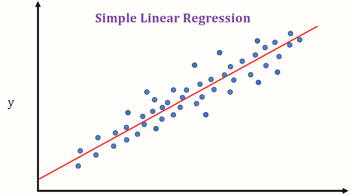
    Linear Regression finds a linear relationship between these features and the target. It essentially draws the “best-fit” straight line (or a hyperplane in higher dimensions) through your data points.

    Types of Linear Regression
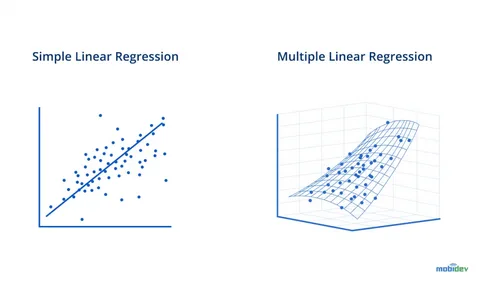
    1. Simple Linear Regression: Involves only one independent variable to predict a dependent variable.
      • Formula: y = mx + b
      • Example: Predicting house price based only on its size.
    2. Multiple Linear Regression: Involves two or more independent variables to predict a dependent variable.
      • Formula: y = b₀ + b₁x₁ + b₂x₂ + ... + bₙxₙ
      • Example: Predicting house price based on size, bedrooms, age, and location.

    The Mathematics Behind Linear Regression: How Does it Find the “Best-Fit” Line?

    How does the algorithm determine which line is the “best”? The answer lies in the Ordinary Least Squares (OLS) method.

    The core idea is to minimize the error between the predicted values and the actual values.

    Key Concepts:

    • The Hypothesis Function: This is the equation of our line.
      • For Simple LR: h(x) = θ₀ + θ₁x (where θ₀ is the intercept, θ₁ is the slope)
      • For Multiple LR: h(x) = θ₀ + θ₁x₁ + θ₂x₂ + ... + θₙxₙ
    • Cost Function (Mean Squared Error – MSE): This function measures how wrong our predictions are. It’s the average of the squared differences between the actual values (y) and the predicted values (h(x)).
      • MSE = (1/n) * Σ(Actualᵢ - Predictedᵢ)²
      • Where n is the number of data points.
    • The Goal: The learning process involves adjusting the parameters (θ₀, θ₁, …, θₙ) to find the values that minimize the MSE. A lower MSE means a better-fitting model.

    Gradient Descent is the optimization algorithm often used to find these optimal parameters. It iteratively adjusts the parameters to move “downhill” on the cost function curve until it finds the minimum value. Think of it as walking down a valley until you reach the lowest point.

    read more about How to Choose the Right Machine Learning Algorithm


    Hands-On Tutorial: Implementing Linear Regression in Python

    Now for the practical part! We will use Python’s powerful scikit-learn library to build a Multiple Linear Regression model.

    Step 1: Importing Necessary Libraries

    We’ll start by importing all the essential tools.

    python

    # For data manipulation and analysis
    import pandas as pd
    import numpy as np
    
    # For data visualization
    import matplotlib.pyplot as plt
    import seaborn as sns
    
    # For machine learning models and tools
    from sklearn.model_selection import train_test_split
    from sklearn.linear_model import LinearRegression
    from sklearn.metrics import mean_absolute_error, mean_squared_error, r2_score
    
    # Magic command for Jupyter notebooks to display plots inline
    %matplotlib inline

    Step 2: Loading and Exploring the Dataset

    For this tutorial, we’ll use a simple sample dataset. In practice, you would load your own CSV file.

    python

    # Create a sample dataset
    data = {
        'Size_sqft': [650, 785, 1200, 1400, 1550, 1800, 2100, 2400, 2750, 3000],
        'Bedrooms': [1, 2, 3, 3, 3, 4, 4, 5, 5, 5],
        'Age': [15, 10, 5, 8, 2, 1, 12, 3, 1, 2],
        'Price': [320000, 385000, 550000, 610000, 650000, 720000, 760000, 800000, 890000, 920000]
    }
    
    # Create a DataFrame
    df = pd.DataFrame(data)
    
    # Display the first 5 rows
    print(df.head())

    Output:

    text

       Size_sqft  Bedrooms  Age   Price
    0        650         1   15  320000
    1        785         2   10  385000
    2       1200         3    5  550000
    3       1400         3    8  610000
    4       1550         3    2  650000

    Step 3: Performing Exploratory Data Analysis (EDA)

    Before modeling, it’s crucial to understand the data.

    python

    # Get a quick statistical summary
    print(df.describe())
    
    # Visualize the relationships between features and target
    sns.pairplot(df)
    plt.show()
    
    # Check the correlation matrix
    plt.figure(figsize=(8, 6))
    sns.heatmap(df.corr(), annot=True, cmap='coolwarm', linewidths=0.5)
    plt.title('Correlation Matrix')
    plt.show()

    The pairplot and correlation matrix help you see which features have the strongest linear relationship with the price (e.g., Size_sqft is likely highly correlated with Price).

    Step 4: Preparing the Data

    We need to split our data into features (X) and target (y), and then into training and testing sets.

    python

    # Define features (X) and target (y)
    X = df[['Size_sqft', 'Bedrooms', 'Age']] # Independent variables
    y = df['Price'] # Dependent variable
    
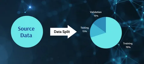
    # Split the data: 80% for training, 20% for testing
    X_train, X_test, y_train, y_test = train_test_split(X, y, test_size=0.2, random_state=42)
    
    print(f"Training set size: {X_train.shape}")
    print(f"Testing set size: {X_test.shape}")

    Step 5: Creating and Training the Model

    This is where we create our Linear Regression model and “fit” it to our training data.

    python

    # Create an instance of the LinearRegression model
    model = LinearRegression()
    
    # Train the model on the training data
    model.fit(X_train, y_train)

    The fit method is where the magic happens—the algorithm learns the parameters (θ₀, θ₁, θ₂, θ₃) that minimize the cost function for our data.

    Step 6: Making Predictions

    Now, let’s use our trained model to make predictions on the test data.

    python

    # Make predictions on the test set
    y_pred = model.predict(X_test)
    
    # Create a DataFrame to compare actual vs predicted values
    results = pd.DataFrame({'Actual': y_test, 'Predicted': y_pred})
    print(results)

    Step 7: Evaluating the Model Performance

    How good is our model? We use evaluation metrics to answer this.

    python

    # Calculate key performance metrics
    mae = mean_absolute_error(y_test, y_pred)
    mse = mean_squared_error(y_test, y_pred)
    rmse = np.sqrt(mse) # Root Mean Squared Error
    r2 = r2_score(y_test, y_pred)
    
    print(f"Mean Absolute Error (MAE): ${mae:,.2f}")
    print(f"Mean Squared Error (MSE): ${mse:,.2f}")
    print(f"Root Mean Squared Error (RMSE): ${rmse:,.2f}")
    print(f"R-squared (R²) Score: {r2:.4f}")

    Interpreting the Metrics:

    • MAE/MSE/RMSE: Measure the average error of the model. Lower values are better. RMSE is especially useful as it is in the same units as the target variable (dollars, in our case).
    • R-squared (R²): Represents the proportion of the variance in the dependent variable that is predictable from the independent variables. It ranges from 0 to 1. A higher value (closer to 1) is better. An R² of 0.95 means 95% of the variation in house prices is explained by our model’s features.

    Step 8: Understanding the Model Coefficients

    Let’s look at the equation our model has created.

    python

    # Get the intercept and coefficients
    print(f"Intercept (θ₀): ${model.intercept_:.2f}")
    
    # Display coefficients alongside their feature names
    coefficients = pd.DataFrame(model.coef_, X.columns, columns=['Coefficient'])
    print(coefficients)

    Interpretation:

    • Intercept (θ₀): The predicted price when all features are zero (often not practically meaningful on its own).
    • Coefficient for ‘Size_sqft’: For every additional square foot, the price increases by [Coefficient Value] dollars, assuming all other features remain constant.
    • Coefficient for ‘Age’: For every additional year in the house’s age, the price decreases by [Coefficient Value] dollars (if the coefficient is negative), assuming all other features remain constant.

    This interpretability is a key strength of Linear Regression.


    Assumptions of Linear Regression

    For the model to be reliable, its key assumptions should be met:

    1. Linearity: The relationship between features and target is linear.
    2. Independence: Observations are independent of each other.
    3. Homoscedasticity: The variance of errors is constant across all levels of the independent variables.
    4. Normality: The errors of the model are normally distributed.
    5. No Multicollinearity: The independent variables are not highly correlated with each other.

    Conclusion: Your First Step into Machine Learning

    Congratulations! You’ve just built and evaluated your first Linear Regression model. You’ve learned:

    • The intuition behind this fundamental algorithm.
    • The core mathematics of how it finds the best-fit line.
    • How to implement it in Python using scikit-learn from start to finish.
    • How to evaluate your model’s performance and interpret its results.

    Linear Regression is a powerful and interpretable tool for prediction. While real-world datasets are often more complex, the principles you’ve learned here are universal. This knowledge forms the bedrock for understanding more advanced algorithms like Logistic Regression, Polynomial Regression, and even Neural Networks.

    Ready to practice? Find a dataset on Kaggle (like the Boston Housing dataset) and try to build your own regression model. The world of machine learning is now at your fingertips.

  • How to Choose the Right Machine Learning Algorithm

    How to Choose the Right Machine Learning Algorithm

    Choosing the right machine learning algorithm is a systematic process based on your problem type, data characteristics, and project constraints—not a random guess. The optimal model balances performance, interpretability, and computational efficiency to deliver real-world value.

    Navigating the vast landscape of machine learning algorithms can be paralyzing. From simple linear regression to complex deep neural networks, the options are endless. Picking the wrong one can lead to months of wasted effort, poor performance, and failed projects. This definitive 2025 guide provides a clear, step-by-step framework to cut through the noise and select the perfect algorithm for your unique challenge.

    read more about Overfitting and Underfitting: The Master Guide to Building Perfect ML Models

    Why Your Choice of Algorithm Matters

    Your algorithm is the engine of your machine learning solution. The right choice leads to:

    • Accurate Predictions: It effectively captures the underlying patterns in your data.
    • Efficient Resource Use: It saves time, computational power, and money.
    • Actionable Insights: It provides results that are interpretable and useful for decision-making.
    • Robust Deployment: It performs reliably in production environments.

    The wrong choice, however, results in inaccurate models, wasted resources, and a solution that never sees the light of day.

    The Ultimate 6-Step Framework to Choose Your Algorithm

    Follow this structured framework to make a confident, data-driven decision.

    Step 1: Define Your Problem Type (The #1 Priority)

    This is the most critical question. The nature of your question dictates the entire category of algorithms you’ll use.

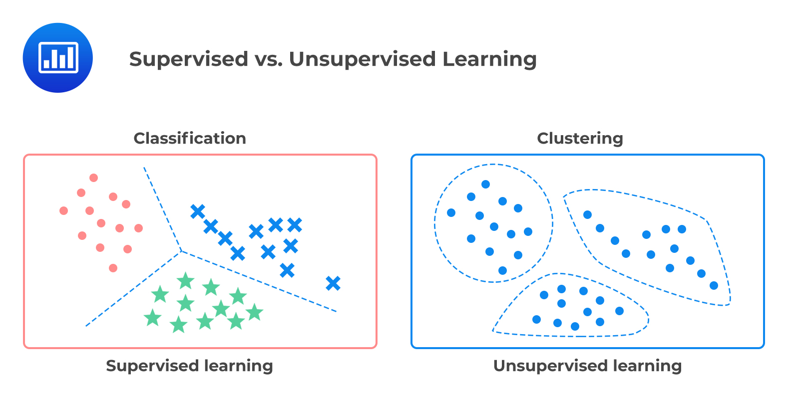
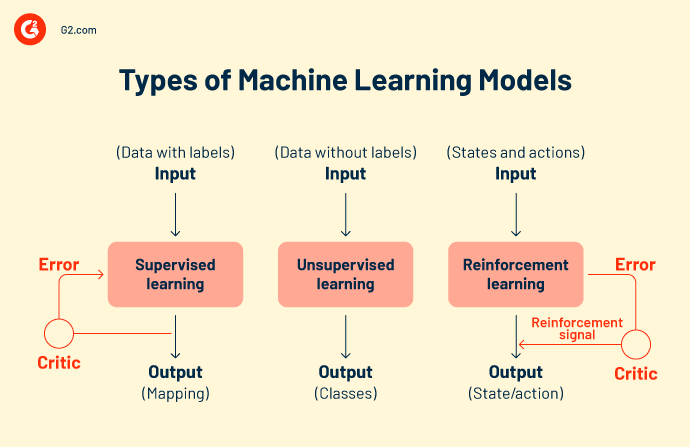
    • Is it Supervised Learning? (Do I have labeled historical data?)
      • Classification: Predicting a category.
        • Binary: Spam vs. Not Spam, Fraud vs. Legitimate.
        • Multi-class: Image recognition (Cat, Dog, Horse), Sentiment Analysis (Positive, Negative, Neutral).
      • Regression: Predicting a continuous value.
        • Examples: House price prediction, sales forecasting, temperature forecasting.
    • Is it Unsupervised Learning? (Do I need to find hidden patterns or structures in unlabeled data?)
      • Clustering: Grouping similar data points.
        • Examples: Customer segmentation, document grouping.
      • Dimensionality Reduction: Reducing the number of features while preserving information.
        • Examples: Data visualization (PCA), feature compression.
      • Anomaly Detection: Identifying rare items or events.
        • Examples: Network intrusion detection, manufacturing defect detection.
    • Is it Reinforcement Learning? (Is an agent learning to make decisions by interacting with an environment?)
      • Examples: Game-playing AI (AlphaGo), robotics, autonomous driving.

    Actionable Takeaway: Write down your problem in a single sentence. This will immediately narrow your options by 80%.

    Step 2: Diagnose Your Data Characteristics

    Your data is the fuel; you must choose an engine that can run on it.

    • Size of Dataset: Is it 1,000 rows or 10 million? Some algorithms scale better than others.
      • Small Data: Models less prone to overfitting are better (e.g., Linear Models, SVM).
      • Large Data: Complex models like Deep Learning and Gradient Boosting can shine.
    • Dimensionality: How many features do you have?
      • High Dimensions: Tree-based models often handle this well. Linear models may require heavy regularization.
    • Linearity: Is the relationship between features and the target linear or complex/non-linear?
      • Linear: Linear Regression, Logistic Regression.
      • Non-linear: Decision Trees, SVM with kernels, Neural Networks.
    • Data Quality: How much noise, missing data, or outliers are present?
      • Noisy Data: Robust models like Random Forest are less affected.
      • Clean Data: You can experiment with more sensitive models.

    Step 3: Establish Your Project Goals & Constraints

    A model that is perfect in theory might be useless in practice due to real-world constraints.

    • Interpretability vs. Performance (The Classic Trade-off):
      • Need to explain “why”? (e.g., loan application denial, medical diagnosis). Choose interpretable models: Linear Models, Decision Trees.
      • Performance is all that matters? (e.g., recommendation system, image classifier). Choose “black box” models: Gradient Boosting, Deep Learning.
    • Training Time vs. Prediction Speed:
      • Need fast training? (e.g., rapid prototyping). Use Linear Models, Naive Bayes.
      • Need fast prediction? (e.g., real-time ad bidding). Use lightweight models like Linear Models. Avoid complex ensembles or large neural networks for high-throughput tasks.
    • Computational Resources:
      • Do you have the GPU power for a large neural network, or do you need a model that runs on a CPU?

    Step 4: Start with a Simple Baseline Model

    Never start with the most complex model. Begin with a simple, interpretable baseline. This establishes a performance floor and provides a sanity check.

    • For Regression: Start with Linear Regression.
    • For Classification: Start with Logistic Regression or a Decision Tree.

    If a complex model can’t significantly beat your simple baseline, it’s probably not worth the added complexity and cost.

    Step 5: Iterate and Evaluate with More Advanced Models

    Once you have a baseline, experiment with more sophisticated algorithms in a structured way.

    • From Linear Models, move to: Support Vector Machines (SVMs), k-Nearest Neighbors (k-NN).
    • Then, try ensemble methods: Random Forest (bagging) and Gradient Boosting Machines (XGBoost, LightGBM, CatBoost) (boosting). These are often the state-of-the-art for tabular data and are an excellent next step.
    • For specific domains:
      • Text/NLP: Consider Naive Bayes for a simple baseline, then move to Neural Networks (RNNs, Transformers).
      • Images/Video: Use Convolutional Neural Networks (CNNs).
      • Sequential/Time-Series Data: Use models like ARIMAProphet, or Recurrent Neural Networks (RNNs/LSTMs).

    Step 6: Validate Rigorously and Compare

    Use a robust validation strategy (like Train/Test Split or k-Fold Cross-Validation) and consistent evaluation metrics to compare models fairly.

    • Classification Metrics: Accuracy, Precision, Recall, F1-Score, ROC-AUC.
    • Regression Metrics: Mean Absolute Error (MAE), Mean Squared Error (MSE), R-squared.

    The model with the best and most consistent performance on your validation set is your winner.

    A Practical Algorithm Cheat Sheet for 2025

    Problem TypeRecommended Algorithms (Start Here)When to Use It
    RegressionLinear Regression, Random Forest, XGBoost/LightGBMPredicting prices, quantities, any continuous value.
    ClassificationLogistic Regression, Random Forest, XGBoost/LightGBMSpam detection, risk analysis, image categorization.
    ClusteringK-Means, DBSCANCustomer segmentation, grouping unlabeled data.
    Dimensionality ReductionPCA (Principal Component Analysis), t-SNEData visualization, feature compression.
    Time Series ForecastingARIMA, Prophet, LSTMsSales forecasting, stock price prediction.
    Computer VisionConvolutional Neural Networks (CNNs)Image classification, object detection.
    Natural Language (NLP)Transformers (BERT, GPT), RNNs/LSTMsSentiment analysis, machine translation.

    Common Pitfalls to Avoid

    • Defaulting to Deep Learning: For most standard tabular data problems, Gradient Boosting (XGBoost) will outperform deep learning and be faster to train. Reserve deep learning for specialized domains (vision, NLP, audio).
    • Ignoring the Business Context: A 95% accurate model that can’t be explained might be less valuable than a 93% accurate model that is fully interpretable.
    • Over-optimizing Too Early: Focus on data quality and feature engineering first. A great dataset with a simple model will beat a poor dataset with a complex model every time.

    Conclusion: Your Path to the Perfect Model

    Choosing the right machine learning algorithm is not about finding a mythical “best” algorithm. It’s about finding the most suitable algorithm for your specific context. By following the six-step framework—Define, Diagnose, Establish, Baseline, Iterate, and Validate—you transform a daunting task into a manageable, systematic process.

    Stop guessing and start building with confidence. Use this guide as your roadmap, and you’ll consistently select models that are not just academically interesting, but powerfully effective in the real world.

  • Feature Engineering: The Ultimate Guide to Building Better Machine Learning Models

    Feature Engineering: The Ultimate Guide to Building Better Machine Learning Models

    Feature Engineering is the art and science of transforming raw data into meaningful features that make machine learning algorithms work effectively. It is a fundamental, often decisive step in the model-building process that directly impacts accuracy, efficiency, and interpretability.

    Imagine trying to teach someone to recognize a cat by showing them random pixels instead of distinct shapes like ears, whiskers, and tails. That’s what asking a machine learning model to learn from poorly constructed data is like. Feature engineering is the process of creating those “ears and whiskers” from your data—the informative, discriminating attributes that allow a model to learn the underlying pattern and make accurate predictions.

    In this comprehensive guide, you will learn exactly what feature engineering is, why it’s arguably the most critical part of a data scientist’s job, and how to implement its core techniques to build superior models.

    read more about Overfitting and Underfitting: The Master Guide to Building Perfect ML Models

    What is Feature Engineering? (A Simple Definition)

    Feature Engineering is the process of using domain knowledge to select, manipulate, and transform raw data into features that can be used in supervised machine learning.

    In simpler terms, your initial dataset is composed of variables or columns. Feature engineering is the act of refining these variables and creating new ones to better represent the underlying problem to the predictive models, leading to improved model performance on unseen data.

    • Raw Data: Date: "2023-10-27"Size: "XL"Price: "$29.99"
    • Engineered Features:
      • From DateDayOfWeek (e.g., 4), IsWeekend (e.g., 0), Month (e.g., 10)
      • From SizeIs_XL (e.g., 1), Numeric_Size (e.g., 3)
      • From PricePrice_Numeric (e.g., 29.99)

    Why Feature Engineering Matters: The Crucial Impact on Your Models

    The quality of your features has a direct, profound impact on the quality of your model’s predictions. Here’s why it’s not just important, but essential.

    1. It Directly Boosts Model Performance

    Well-engineered features are the single biggest factor in improving a model’s accuracy. A simple model with excellent features will consistently outperform a complex, state-of-the-art model with poor features. The model can focus on the true signals in the data rather than struggling to decipher noisy or irrelevant inputs.

    2. It Aligns Data with Algorithm Requirements

    Many machine learning algorithms have inherent assumptions. Linear models, for instance, assume a linear relationship between features and the target variable. Feature engineering allows you to create features that meet these assumptions (e.g., by transforming non-linear relationships).

    3. It Improves Model Efficiency and Simplicity

    By creating more informative features, you can often achieve the same or better performance with a simpler model. Furthermore, techniques like feature selection reduce the number of input features (dimensionality), which drastically cuts down training time and computational cost.

    4. It Enhances Model Generalization

    A model trained on irrelevant or redundant features is prone to overfitting—it memorizes the noise in the training data instead of learning the generalizable pattern. Proper feature engineering, especially through selection and creation of robust features, helps the model focus on what truly matters, improving its performance on new, unseen data.

    Core Techniques of Feature Engineering: A Practical Toolkit

    Feature engineering can be broken down into several key areas. Let’s explore the most critical techniques with practical examples.

    1. Handling Missing Data

    Real-world data is messy. Missing values are common and can break many algorithms.

    • Deletion: Remove rows or columns with missing values. (Useful only when the missing data is random and a small percentage).
    • Imputation (Numerical): Fill missing values with the mean, median, or mode. For time-series data, use forward-fill or backward-fill.
    • Imputation (Categorical): Create a new category like “Unknown” or “Missing” to capture the fact that the value was not present.

    2. Encoding Categorical Variables

    Most algorithms require numerical input. Encoding transforms categories into numbers.

    • One-Hot Encoding: Creates a new binary (0/1) column for each category. Ideal for nominal data (categories with no order, e.g., “Red,” “Blue,” “Green”).
    • Label Encoding: Assigns a unique integer to each category (e.g., “Red”=0, “Blue”=1). Use with caution, as it can imply an order that doesn’t exist. Best for ordinal data (e.g., “Low,” “Medium,” “High”).

    3. Feature Scaling and Normalization

    When features have different scales (e.g., Age: 0-100, Salary: 50,000-200,000), models like SVMs, K-Nearest Neighbors, and Gradient Descent-based algorithms can be biased toward the larger-scale features.

    • Standardization (Z-Score Normalization): Transforms data to have a mean of 0 and a standard deviation of 1. (x - mean) / std
    • Min-Max Scaling: Scales data to a fixed range, usually [0, 1]. (x - min) / (max - min)

    4. Creating New Features (Feature Creation)

    This is where domain expertise truly shines. You create new, more informative features from existing ones.

    • From Dates: Extract YearMonthDayOfWeekIsWeekendIsHoliday.
    • From Text: Create features like TextLengthWordCountSentimentScore.
    • Aggregations: For customer data, create features like TotalPurchasesAverageSpendDaysSinceLastPurchase.
    • Polynomial Features: Create interaction terms (e.g., Feature_A * Feature_B) to help linear models capture non-linear relationships.

    5. Binning / Discretization

    Transforming continuous numerical features into categorical bins can help models learn non-linear patterns and handle outliers.

    • Example: Convert Age (continuous) into Age_Group (categorical: “0-17”, “18-25”, “26-40”, “40+”).

    6. Feature Selection

    Not all features are useful. Redundant or irrelevant features add noise and complexity. The goal is to select the most predictive subset.

    • Filter Methods: Use statistical measures (e.g., Correlation, Chi-Squared) to select the best features.
    • Wrapper Methodshttps://www.geeksforgeeks.org/machine-learning/wrapper-methods-feature-selection/: Use a model’s performance as the evaluation criteria (e.g., Recursive Feature Elimination).
    • Embedded Methods: Algorithms like Lasso (L1 regularization) and Random Forests have built-in feature selection.

    The Feature Engineering Workflow: A Step-by-Step Process

    A structured approach ensures you don’t miss critical steps.
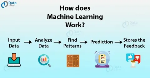
    1. Data Discovery & Domain Learning: Understand what each feature represents and its business context.
    2. Data Cleaning: Handle missing values and obvious outliers.
    3. Exploratory Data Analysis (EDA): Visualize distributions, correlations, and relationships with the target variable.

    4. Baseline Model: Train a simple model on raw features to establish a performance baseline.
    5. Iterative Engineering & Selection: Apply the techniques above. Create new features, encode, scale, and then select the best ones.
    6. Final Model Training & Validation: Train your model on the final engineered feature set and validate its performance on a hold-out test set.

    Common Pitfalls to Avoid

    • Data Leakage: Never use information from your test set (like its mean) to engineer features in your training set. Always fit imputers and scalers on the training data only.
    • Over-Engineering: Creating too many complex, highly specific features can lead to overfitting. Keep it simple and interpretable where possible.
    • Ignoring Domain Knowledge: The most powerful features often come from a deep understanding of the problem, not just automated techniques.

    Conclusion: Master Feature Engineering, Master Machine Learning

    While the allure of complex algorithms is strong, the true leverage in machine learning often comes from the thoughtful, creative, and systematic practice of feature engineering. It is the bridge that connects raw data to intelligent algorithms. By investing time in crafting high-quality features, you build a solid foundation for your models, enabling them to not just function, but to excel.

    Start treating your features as a primary asset. Experiment with the techniques outlined in this guide, lean on domain expertise, and watch as your model performance reaches new heights.


  • Overfitting and Underfitting: The Master Guide to Building Perfect ML Models

    Overfitting and Underfitting: The Master Guide to Building Perfect ML Models

    In the world of Machine Learning (ML), your ultimate goal is simple: build a model that performs well on new, unseen data. This ability is called generalization. However, two formidable barriers stand between you and this goal, haunting every data scientist from beginner to expert—overfitting and underfitting.

    Understanding these concepts is not just academic; it’s the practical core of building robust, reliable, and effective ML models. This definitive guide will take you from a conceptual understanding to a practical mastery of diagnosing, resolving, and preventing overfitting and underfitting.

    The Core Problem: The Bias-Variance Tradeoff

    To truly grasp overfitting and underfitting, you must first understand their root cause: the Bias-Variance Tradeoff. This fundamental concept describes the tension between a model’s simplicity and its complexity.

    Let’s break it down:

    • Bias: Error due to overly simplistic assumptions in the learning algorithm. A high-bias model is like a student who only skimmed the chapter titles; they miss important nuances and details, leading to inaccurate predictions on both training and new data. This is Underfitting.
    • Variance: Error due to excessive complexity in the learning algorithm. A high-variance model is like a student who memorizes the textbook word-for-word, including the footnotes and page numbers. They perform perfectly on the training material but fail miserably on a exam that asks the same concepts in a different way. This is Overfitting.

    The “tradeoff” is this: as you reduce bias (make the model more complex), variance tends to increase, and vice-versa. The art of machine learning is finding the sweet spot between the two.

    learn more about Top 10 Free Datasets for Practicing Machine Learning in 2025

    What is Underfitting?

    Underfitting occurs when a model is too simple to capture the underlying pattern or trend in the data.

    The Analogy: Imagine trying to fit a straight line (a simple model) to a dataset that clearly follows a curved, parabolic path. The straight line will be inaccurate everywhere because it’s the wrong tool for the job. It’s like using a butter knife to cut down a tree—it’s fundamentally not up to the task.

    Causes of Underfitting:

    1. Excessively Simple Model: Using a linear model for a non-linear problem.
    2. Too Little Training Time: Stopping the training process too early (e.g., in deep learning).
    3. Heavily Noisy Data: The signal is too weak compared to the noise.
    4. Extreme Regularization: Applying too much regularization, which over-penalizes complexity.

    How to Diagnose Underfitting:

    • Performance Metrics: The model performs poorly on the training data and equally poorly (or worse) on the testing/validation data.
    • Visual Cues (for low dimensions): The model’s decision boundary or regression line fails to follow the natural flow of the data points.

    What is Overfitting?

    Overfitting occurs when a model is excessively complex, learning not only the underlying pattern but also the noise and random fluctuations in the training data.

    The Analogy: The model is like a tailor who creates a suit that fits one specific client’s body perfectly, down to the last mole and slight slouch. However, if anyone else tries to wear that suit, it won’t fit at all. The suit has “memorized” the client instead of learning the general pattern of a human form.

    Causes of Overfitting:

    1. Excessively Complex Model: Using a deep neural network with millions of parameters for a simple task.
    2. Training for Too Long: In iterative algorithms (like neural networks), the model starts to “memorize” the training data over time.
    3. Too Many Features / High Dimensionality: Having a vast number of features without enough data points to support them (the “curse of dimensionality”).
    4. Insufficient Training Data: The model doesn’t have enough examples to generalize from.

    The Battle Plan: How to Prevent and Fix Overfitting & Underfitting

    Here are the key techniques used by ML practitioners to find the perfect balance.

    Strategies to Combat UNDERFITTING:

    1. Increase Model Complexity: Switch from a linear model to a non-linear one (e.g., Decision Trees, SVM with non-linear kernels, Neural Networks).
    2. Add More Relevant Features: Perform feature engineering to create more informative input variables for the model.
    3. Reduce Regularization: Regularization techniques (like L1/L2) penalize complexity. Reducing their strength allows the model to become more complex.
    4. Train for Longer: Allow the model more time to learn from the data, especially for iterative algorithms like gradient descent.

    Strategies to Combat OVERFITTING:

    1. Cross-Validation: Use techniques like k-fold cross-validation to get a more robust estimate of model performance and ensure it generalizes well.
    2. Gather More Training Data: This is often the most effective method. More data helps the model distinguish the true signal from the noise.
    3. Feature Selection/Reduction: Reduce the number of features using techniques like PCA (Principal Component Analysis) or by selecting only the most important features.
    4. Regularization (L1 & L2): Add a penalty to the model’s loss function for having large coefficients. This discourages the model from becoming too complex.
      • L1 (Lasso): Can shrink some coefficients to zero, effectively performing feature selection.
      • L2 (Ridge): Shrinks all coefficients proportionally.
    5. Ensemble Methods: Use methods like Bagging (e.g., Random Forest) that combine multiple weak models to reduce variance. A Random Forest is essentially a large collection of de-correlated Decision Trees, which are individually prone to overfitting, but together are very robust.
    6. Early Stopping: For iterative learners (like Neural Networks), stop the training process as soon as the performance on the validation set starts to degrade.
    7. Pruning: For Decision Trees, cut back the branches of the tree that have little power in predicting the target variable, simplifying the model.
    8. Dropout: A specific technique for Neural Networks where randomly selected neurons are “dropped out” during training, preventing the network from becoming over-reliant on any single neuron.

    Summary Table: Overfitting vs. Underfitting at a Glance

    FeatureOverfittingUnderfitting
    Model ComplexityToo HighToo Low
    Performance on Training DataExcellentPoor
    Performance on Test DataPoorPoor
    Captures Noise?YesNo
    Captures Underlying Pattern?No (only memorizes)No (too simple)
    AnalogyMemorizing the textbookSkimming the textbook
    Primary Error TypeHigh VarianceHigh Bias

    Conclusion: The Path to the “Just Right” Model

    Mastering overfitting and underfitting is a non-negotiable skill in machine learning. It’s the continuous process of navigating the bias-variance tradeoff to find the “Goldilocks Zone” where your model is neither too simple nor too complex.

    The key to success is rigorous evaluation using a hold-out validation set or cross-validation, and a toolkit of techniques like regularization, ensemble methods, and feature engineering. By systematically diagnosing the symptoms and applying the correct remedies, you can build models that don’t just look good on paper but deliver real, reliable value in the unpredictable real world.

    Your Next Step: Open your favorite ML library (like Scikit-learn), train a simple and a complex model on a dataset, and plot the learning curves. Seeing the gap between training and validation error emerge firsthand is the best way to solidify these critical concepts.

  • Top 10 Free Datasets for Practicing Machine Learning in 2025

    Top 10 Free Datasets for Practicing Machine Learning in 2025

    Finding high-quality, free datasets is the cornerstone of machine learning mastery. As we approach 2025, the landscape of available data continues to evolve, offering unprecedented opportunities for hands-on learning and portfolio development.

    This definitive guide curates the best free datasets for machine learninghttps://365datascience.com/trending/public-datasets-machine-learning/ in 2025, specifically chosen for their educational value, real-world relevance, and ability to help you build job-ready skills. Whether you’re a complete beginner or an experienced practitioner, these datasets will provide the perfect foundation for your machine learning journey.

    Why Quality Datasets Matter for ML Success

    Before diving into our curated list, understand that working with the right datasets accelerates your learning by:

    • Building practical experience with real-world data challenges
    • Developing portfolio projects that impress employers
    • Understanding data preprocessing nuances across different domains
    • Testing multiple algorithms on diverse problem types
    • Learning industry-standard tools and workflows

    Our 2025 Dataset Selection Criteria

    Each dataset in this list meets these rigorous standards:

    • ✅ Completely free with easy access
    • ✅ Appropriate size for different skill levels
    • ✅ High data quality and cleanliness
    • ✅ Diverse problem types and domains
    • ✅ Active community support and documentation
    • ✅ Real-world relevance and practical applications

    The Top 10 Free Machine Learning Datasets for 2025

    1. Titanic: Machine Learning from Disaster

    Ideal For: Absolute Beginners | Classification Problems

    Dataset Overview:

    • Problem Type: Binary Classification
    • Records: 891 training, 418 test
    • Features: 11 passenger attributes
    • Goal: Predict passenger survival

    Why It’s Perfect for 2025:
    The Titanic dataset remains the “Hello World” of machine learning for good reason. It introduces fundamental concepts like feature engineering, missing value handling, and model evaluation in a digestible package.

    Learning Opportunities:

    • Data cleaning and imputation
    • Feature engineering (title extraction, family size)
    • Binary classification algorithms
    • Cross-validation techniques

    Access Method:

    python

    # Through Kaggle API
    kaggle competitions download -c titanic
    # Or directly from sklearn
    from sklearn.datasets import fetch_openml
    titanic = fetch_openml('titanic', version=1, as_frame=True)

    2. California Housing Prices

    Ideal For: Intermediate Learners | Regression Problems

    Dataset Overview:

    • Problem Type: Multivariate Regression
    • Records: 20,640
    • Features: 8 economic and geographic attributes
    • Goal: Predict median house values

    Why It’s Perfect for 2025:
    This dataset introduces spatial analysis and economic forecasting—highly relevant skills for 2025 job markets in real estate tech and geographic AI applications.

    Learning Opportunities:

    • Handling geographical data
    • Feature scaling and transformation
    • Regression model evaluation
    • Dealing with skewed distributions

    Access Method:

    python

    from sklearn.datasets import fetch_california_housing
    housing = fetch_california_housing()
    df = pd.DataFrame(housing.data, columns=housing.feature_names)

    3. Iris Species Classification

    Ideal For: Beginners | Multi-class Classification

    Dataset Overview:

    • Problem Type: Multi-class Classification
    • Records: 150
    • Features: 4 botanical measurements
    • Goal: Classify iris flower species

    Why It’s Perfect for 2025:
    While simple, Iris remains valuable for understanding clustering and classification fundamentals. It’s perfect for testing new algorithms quickly.

    Learning Opportunities:

    • Data visualization and EDA
    • Clustering algorithms (K-means)
    • Multi-class classification
    • Model interpretability

    Access Method:

    python

    from sklearn.datasets import load_iris
    iris = load_iris()
    X, y = iris.data, iris.target

    4. Credit Card Fraud Detection

    Ideal For: Advanced Practitioners | Imbalanced Classification

    Dataset Overview:

    • Problem Type: Binary Classification (Highly Imbalanced)
    • Records: 284,807 transactions
    • Features: 28 PCA-transformed numerical features
    • Goal: Detect fraudulent transactions

    Why It’s Perfect for 2025:
    With digital payment fraud increasing, this dataset teaches crucial skills in handling severe class imbalance—a common challenge in real-world ML.

    Learning Opportunities:

    • Handling imbalanced datasets
    • Anomaly detection techniques
    • Precision-Recall tradeoffs
    • Cost-sensitive learning

    Access Method:

    python

    # Download from Kaggle
    kaggle datasets download -d mlg-ulb/creditcardfraud
    # Or use direct URL
    import pandas as pd
    url = "https://datahub.io/mlg-ulb/creditcardfraud/r/creditcard.csv"
    df = pd.read_csv(url)

    5. Wine Quality Dataset

    Ideal For: Intermediate | Multi-class & Regression

    Dataset Overview:

    • Problem Type: Multi-class Classification or Regression
    • Records: 4,898 (red), 1,599 (white)
    • Features: 11 chemical properties
    • Goal: Predict wine quality scores (0-10)

    Why It’s Perfect for 2025:
    This dataset bridges classification and regression, perfect for understanding how problem framing affects model selection and performance.

    Learning Opportunities:

    • Regression to classification conversion
    • Feature correlation analysis
    • Multi-output regression
    • Model ensemble techniques

    Access Method:

    python

    import pandas as pd
    red_wine = pd.read_csv('https://archive.ics.uci.edu/ml/machine-learning-databases/wine-quality/winequality-red.csv', sep=';')
    white_wine = pd.read_csv('https://archive.ics.uci.edu/ml/machine-learning-databases/wine-quality/winequality-white.csv', sep=';')

    6. MNIST Handwritten Digits

    Ideal For: Computer Vision Beginners | Image Classification

    Dataset Overview:

    • Problem Type: Multi-class Image Classification
    • Records: 70,000 grayscale images
    • Features: 28×28 pixel arrays (784 features)
    • Goal: Classify handwritten digits (0-9)

    Why It’s Perfect for 2025:
    MNIST remains the gateway to computer vision, now enhanced by modern deep learning frameworks. Perfect for learning neural networks and CNN architectures.

    Learning Opportunities:

    • Image preprocessing
    • Neural network implementation
    • Convolutional Neural Networks (CNNs)
    • Model performance benchmarking

    Access Method:

    python

    from tensorflow.keras.datasets import mnist
    (X_train, y_train), (X_test, y_test) = mnist.load_data()

    7. COVID-19 Open Research Dataset (CORD-19)

    Ideal For: NLP Enthusiasts | Text Mining

    Dataset Overview:

    • Problem Type: Natural Language Processing
    • Records: 1,000,000+ scholarly articles
    • Features: Full-text research papers, abstracts, metadata
    • Goal: Various NLP tasks (classification, summarization, QA)

    Why It’s Perfect for 2025:
    This real-time dataset teaches modern NLP techniques on relevant scientific literature, bridging healthcare and AI—a growing field in 2025.

    Learning Opportunities:

    • Text preprocessing and cleaning
    • Topic modeling (LDA, BERTopic)
    • Document classification
    • Named Entity Recognition (NER)

    Access Method:

    python

    # Through Kaggle API
    kaggle datasets download -d allen-institute-for-ai/CORD-19-research-challenge

    8. NYC Taxi Trip Duration

    Ideal For: Intermediate/Advanced | Time Series & Regression

    Dataset Overview:

    • Problem Type: Regression with Temporal Features
    • Records: 1,458,644 taxi trips
    • Features: 11 trip attributes including timestamps
    • Goal: Predict taxi trip duration

    Why It’s Perfect for 2025:
    Time series forecasting and geospatial analysis are critical skills for 2025 job markets in logistics, transportation, and urban planning.

    Learning Opportunities:

    • Time feature engineering
    • Geospatial data handling
    • Advanced regression techniques
    • Feature importance analysis

    Access Method:

    python

    kaggle competitions download -c nyc-taxi-trip-duration

    9. Fashion-MNIST

    Ideal For: Computer Vision | Multi-class Classification

    Dataset Overview:

    • Problem Type: Image Classification
    • Records: 70,000 grayscale images
    • Features: 28×28 pixel arrays
    • Goal: Classify fashion products into 10 categories

    Why It’s Perfect for 2025:
    As a modern replacement for MNIST, Fashion-MNIST offers more realistic challenges for e-commerce and retail AI applications.

    Learning Opportunities:

    • Advanced CNN architectures
    • Transfer learning
    • Data augmentation
    • Model interpretability for images

    Access Method:

    python

    from tensorflow.keras.datasets import fashion_mnist
    (X_train, y_train), (X_test, y_test) = fashion_mnist.load_data()

    10. Google Play Store Apps

    Ideal For: Business Analytics | Regression & Classification

    Dataset Overview:

    • Problem Type: Regression & Multi-class Classification
    • Records: 10,000+ Android apps
    • Features: 13 app attributes (category, reviews, size, etc.)
    • Goal: Predict app ratings or success metrics

    Why It’s Perfect for 2025:
    This dataset bridges machine learning and business intelligence, teaching how to derive commercial insights from app data.

    Learning Opportunities:

    • Business metric forecasting
    • Categorical feature handling
    • Multi-modal data analysis
    • Recommendation system prototyping

    Access Method:

    python

    import pandas as pd
    url = "https://raw.githubusercontent.com/amankharwal/Website-data/master/googleplaystore.csv"
    df = pd.read_csv(url)
    learn more about 5 Essential Python Libraries to Start Your Machine Learning Journeyhttps://codetinkerai.blog/wp-admin/post.php?post=260&action=edit

    2025 Learning Roadmap Using These Datasets

    Beginner Path (0-3 Months)

    1. Start with: Iris → Titanic → California Housing
    2. Focus: Data cleaning, basic algorithms, model evaluation
    3. Goal: Build confidence with foundational concepts

    Intermediate Path (3-6 Months)

    1. Progress to: Wine Quality → Fashion-MNIST → Google Play Store
    2. Focus: Feature engineering, advanced algorithms, hyperparameter tuning
    3. Goal: Develop portfolio-worthy projects

    Advanced Path (6+ Months)

    1. Tackle: Credit Card Fraud → NYC Taxi → CORD-19
    2. Focus: Real-world challenges, ensemble methods, deep learning
    3. Goal: Prepare for industry roles and competitions

    Where to Find More Datasets in 2025

    Primary Sources:

    • Kaggle Datasets: Largest community with constant updates
    • UCI Machine Learning Repository: Academic classic with curated datasets
    • Google Dataset Search: Meta-search across multiple sources
    • Government Data Portals: Real-world data from various agencies
    • Hugging Face Datasets: Modern platform for NLP and beyond

    Emerging 2025 Platforms:

    • Data.gov.sg (Singapore)
    • EU Open Data Portal
    • AWS Data Exchange
    • Microsoft Research Open Data

    Best Practices for Dataset Usage in 2025

    1. Always Check Licenses: Ensure commercial use permissions
    2. Validate Data Quality: Check for biases and completeness
    3. Document Your Process: Create reproducible workflows
    4. Respect Privacy: Anonymize sensitive information
    5. Contribute Back: Share your cleaned versions and insights

    Conclusion: Start Your Machine Learning Journey Today

    The datasets highlighted in this guide represent the best free machine learning datasets for 2025, carefully selected to provide maximum learning value across different skill levels and domains.

    Remember that consistent practice with diverse datasets is the fastest path to machine learning mastery. Each dataset you work with builds another layer of practical experience that separates hobbyists from professionals.

    Your Action Plan:

    1. Choose one dataset matching your current skill level
    2. Set clear learning objectives for each project
    3. Document your work in a GitHub portfolio
    4. Share your findings with the community
    5. Progress to more challenging datasets

    The field of machine learning continues to evolve rapidly, but the fundamentals remain constant. By mastering these essential datasets, you’ll build a strong foundation that will serve you throughout 2025 and beyond.


  • Supervised vs Unsupervised Learning: The Plain English Guide for 2025

    Supervised vs Unsupervised Learning: The Plain English Guide for 2025

    In the rapidly evolving landscape of artificial intelligence, understanding the fundamental difference between supervised and unsupervised learning remains crucial for anyone looking to grasp how machines truly learn. As we move into 2025, these concepts have become more relevant than ever, powering everything from advanced healthcare diagnostics to personalized shopping experiences.

    If you’ve ever wondered how Netflix knows exactly what you want to watch next, or how your bank detects fraudulent transactions before you even notice, you’re encountering the practical applications of these two machine learning paradigms.

    This comprehensive guide will demystify supervised vs unsupervised learninghttps://cloud.google.com/discover/supervised-vs-unsupervised-learning using clear explanations, relatable analogies, and real-world examples that show how these technologies are shaping our world in 2025.

    The Core Difference: The Answer Key Analogy

    The simplest way to understand supervised vs unsupervised learning is through a school analogy:

    • Supervised Learning = Learning with an Answer Key
      Imagine studying for a test with a textbook that includes both practice questions AND answers. You can check your work, learn from mistakes, and gradually understand the patterns.
    • Unsupervised Learning = Discovering Patterns Without Guidance
      Now imagine being given a dataset with no labels or answers—like being handed a thousand different leaves and being asked to organize them without any botanical knowledge. You’d naturally group them by color, shape, or size based on the patterns you observe.

    This fundamental difference—the presence or absence of labeled data—defines the entire supervised vs unsupervised learning paradigm.

    What is Supervised Learning? The Guided Approach

    Supervised learning involves training algorithms using labeled datasets, where each example includes both input data and the correct output. The model learns to map inputs to outputs, gradually improving its ability to make accurate predictions on new, unseen data.

    Key Characteristics for 2025:

    • ✅ Uses labeled training data
    • ✅ Direct feedback mechanism
    • ✅ Predicts outcomes/classifications
    • ✅ Performance is easily measurable
    • ✅ Requires human intervention for labeling

    Real-World Supervised Learning Examples in 2025:

    1. Medical Diagnosis Systems
      Modern healthcare AI uses supervised learning to analyze medical images. Radiologists label thousands of X-rays, MRIs, and CT scans as “healthy” or showing specific conditions. The trained model can then assist doctors in detecting diseases like cancer with remarkable accuracy.
    2. Autonomous Vehicle Navigation
      Self-driving cars use supervised learning to recognize traffic signs, pedestrians, and other vehicles. They’re trained on millions of labeled images, learning to identify stop signs, traffic lights, and potential hazards.
    3. Sentiment Analysis for Customer Service
      Companies train models on customer messages labeled as “positive,” “negative,” or “neutral” to automatically route complaints, measure satisfaction, and identify emerging issues.

    What is Unsupervised Learning? The Pattern Detective

    Unsupervised learning algorithms work with unlabeled data, searching for inherent patterns, structures, or groupings without any predefined categories or guidance.

    Key Characteristics for 2025:

    • 🔍 Works with unlabeled data
    • 🔍 No direct feedback mechanism
    • 🔍 Discovers hidden patterns
    • 🔍 Performance can be subjective
    • 🔍 Minimal human intervention needed

    Real-World Unsupervised Learning Examples in 2025:

    1. Advanced Customer Segmentation
      E-commerce platforms analyze purchasing behavior to identify micro-segments of customers they didn’t know existed, enabling hyper-personalized marketing campaigns that go beyond traditional demographics.
    2. Anomaly Detection in Cybersecurity
      Systems monitor network traffic patterns to identify unusual behavior that could indicate security breaches, zero-day attacks, or internal threats—without knowing what “normal” looks like in advance.
    3. Genomic Pattern Discovery
      Researchers use unsupervised learning to identify previously unknown genetic markers and biological patterns, accelerating drug discovery and personalized medicine.

    Supervised vs Unsupervised Learning: 2025 Comparison Table

    AspectSupervised LearningUnsupervised Learning
    Data RequirementsLabeled dataRaw, unlabeled data
    Computational ComplexityGenerally higherOften lower
    Primary GoalPrediction & ClassificationPattern discovery & insight generation
    Common AlgorithmsRandom Forests, Neural Networks, SVMK-means, DBSCAN, Autoencoders
    InterpretabilityMore interpretable resultsCan be harder to interpret
    Human InvolvementHigh (for labeling)Minimal
    2025 ApplicationsDiagnostic AI, Fraud detection, Predictive maintenanceMarket basket analysis, Social network analysis, Drug discovery

    When to Use Each Approach: A Practical 2025 Guide

    Choose Supervised Learning When:

    • You have clearly labeled historical data
    • You need to make specific predictions or classifications
    • Accuracy and precision are critical
    • You can afford the time/cost of data labeling
    • The problem has well-defined outcomes

    Example: Predicting customer churn for a subscription service where you have historical data showing which customers left and why.

    Choose Unsupervised Learning When:

    • You’re exploring unknown data patterns
    • Data labeling is impractical or expensive
    • You want to discover hidden segments or relationships
    • You’re dealing with completely new problem domains
    • You need to reduce data dimensionality

    Example: Analyzing user behavior on a new social media platform to discover natural user types and usage patterns.

    The Emerging Middle Ground: Semi-Supervised and Self-Supervised Learning

    As we move further into 2025, the lines between supervised and unsupervised learning are blurring with hybrid approaches:

    read more about Top 10 Future Technologies That Will Change the Worldhttps://codetinkerai.blog/wp-admin/post.php?post=274&action=edit

    Semi-Supervised Learning

    This approach uses a small amount of labeled data combined with a large amount of unlabeled data. It’s particularly useful when obtaining fully labeled datasets is expensive or time-consuming.

    2025 Application: Medical image analysis where experts label a small subset of images, and the model learns from both labeled and unlabeled data.

    Self-Supervised Learning

    Models generate their own labels from the data itself, creating a form of supervised learning without human intervention.

    2025 Application: Large language models like GPT-4 that learn by predicting the next word in a sentence, using the surrounding context as implicit labels.

    Common Challenges and Solutions in 2025

    Supervised Learning Challenges:

    • Data Labeling Costs: Automated labeling tools and crowd-sourcing platforms are reducing this burden
    • Overfitting: Advanced regularization techniques and more sophisticated validation methods
    • Label Quality: Improved data curation pipelines and quality assurance protocols

    Unsupervised Learning Challenges:

    • Evaluation Difficulty: New metrics and visualization tools for assessing cluster quality
    • Interpretability: Enhanced explanation algorithms and visualization dashboards
    • Scalability: Distributed computing and optimized algorithms for large datasets

    Getting Started in 2025: Your Learning Path

    For Supervised Learning:

    1. Start with classification using scikit-learn’s built-in datasets
    2. Practice with real-world datasets from Kaggle
    3. Learn about train-test splits and cross-validation
    4. Explore deep learning frameworks like TensorFlow or PyTorch

    For Unsupervised Learning:

    1. Begin with clustering algorithms like K-means
    2. Experiment with dimensionality reduction using PCA
    3. Work with anomaly detection datasets
    4. Explore neural network-based approaches like autoencoders

    The Future Beyond 2025

    The distinction between supervised and unsupervised learning will continue to evolve as:

    • Reinforcement learning bridges the gap between both approaches
    • Foundation models demonstrate unprecedented few-shot learning capabilities
    • Neuromorphic computing enables more brain-like learning patterns
    • Federated learning allows models to learn from decentralized data while preserving privacy

    Conclusion: Two Sides of the Same Coin

    Understanding the difference between supervised and unsupervised learning is fundamental to grasping how artificial intelligence systems work. While they approach learning from different directions, both are essential tools in the modern AI toolkit.

    As we progress through 2025, the most powerful applications will likely combine both approaches, using unsupervised learning to discover patterns and supervised learning to make precise predictions based on those discoveries.

    Whether you’re a business leader making technology decisions, a developer building AI applications, or simply someone curious about how modern technology works, recognizing when to apply supervised vs unsupervised learning will help you better understand and leverage the AI revolution shaping our world.

  • How to Prepare Your Data for Machine Learning: A Complete 2025 Step-by-Step Guide

    How to Prepare Your Data for Machine Learning: A Complete 2025 Step-by-Step Guide

    Data preparation remains the most critical—and often most overlooked—phase of any successful machine learning project. As we enter 2025, studies show that data scientists still spend 45-60% of their time on data preparation tasks, with advanced organizations reporting that proper data preprocessing can improve model accuracy by up to 70%.

    This definitive 2025 guide will walk you through the exact, battle-tested framework that top AI teams use to transform raw, messy data into a clean, machine-ready dataset. Whether you’re a beginner working on your first Kaggle competition or a seasoned professional building enterprise AI systems, this step-by-step tutorial will give you the complete data preparation toolkit for 2025.

    Why Data Preparation Matters More Than Ever in 2025

    The machine learning landscape has evolved dramatically, but one principle remains unchanged: garbage in, garbage out. Proper data preparation in 2025 is crucial because:

    • Foundation Models & LLMs still require clean, structured data for fine-tuning
    • AI Regulations (EU AI Act, US Executive Orders) mandate data quality and fairness
    • Edge AI Deployment demands optimized, efficient data pipelines
    • Multi-Modal Learning requires sophisticated data integration techniques
    • AutoML Systems perform better with well-prepared input data

    Think of data preparation as the difference between building on solid ground versus quicksand—your model’s entire success depends on this foundation.

    The 8-Step Data Preparation Framework for 2025

    Here’s the complete, updated framework that incorporates the latest 2025 best practices:

    Step 1: Data Collection & Modern Data Stack Integration

    2025 Update: Data sources have multiplied, requiring sophisticated integration strategies.

    Key Activities:

    • Multi-source aggregation (APIs, cloud storage, data lakes, real-time streams)
    • Data lineage tracking for compliance and reproducibility
    • Initial data profiling to understand volume, variety, and velocity
    • Privacy-preserving collection following GDPR/CCPA guidelines

    2025 Tools & Techniques:

    python

    # Modern data collection with Python
    import pandas as pd
    import pyarrow.parquet as pq
    from sklearn.datasets import fetch_openml
    import great_expectations as ge
    
    # Collect from multiple sources
    df_api = pd.read_json('https://api.yourdata.com/v2/records')
    df_cloud = pd.read_parquet('s3://your-bucket/data-2025.parquet')
    df_local = pd.read_csv('local_dataset.csv')
    
    # Data quality assessment
    df_ge = ge.from_pandas(df_api)
    results = df_ge.validate()

    Step 2: Comprehensive Data Understanding & Profiling

    2025 Update: Automated EDA tools have become standard, with AI-assisted insights.

    Key Activities:

    • Automated data profiling with AI-powered tools
    • Data quality assessment scoring
    • Domain context integration with business experts
    • Bias and fairness detection in initial datasets

    Modern EDA Approach:

    python

    # 2025 Automated EDA
    from ydata_profiling import ProfileReport
    import sweetviz as sv
    import dataprep
    
    # Generate comprehensive profile
    profile = ProfileReport(df, title="Data Profile 2025")
    profile.to_file("data_profile.html")
    
    # Automated bias detection
    from aif360.datasets import BinaryLabelDataset
    from aif360.metrics import DatasetMetric
    
    # Check for protected attribute bias
    protected_dataset = BinaryLabelDataset(...)
    metric = DatasetMetric(protected_dataset, ...)
    print(f"Disparate impact: {metric.disparate_impact()}")

    Step 3: Advanced Data Cleaning & Quality Enhancement

    2025 Update: ML-powered cleaning tools and synthetic data generation for missing values.

    Key Activities:

    • AI-powered imputation using neural networks and generative methods
    • Automated outlier detection with ensemble methods
    • Cross-validation aware cleaning to prevent data leakage
    • Data augmentation for small datasets

    Modern Cleaning Techniques:

    python

    from sklearn.experimental import enable_iterative_imputer
    from sklearn.impute import IterativeImputer
    from sklearn.ensemble import RandomForestRegressor
    from fancyimpute import KNN, NuclearNormMinimization
    
    # Advanced imputation strategies
    imputer = IterativeImputer(estimator=RandomForestRegressor(), 
                              max_iter=10, random_state=42)
    df_imputed = imputer.fit_transform(df)
    
    # Automated outlier detection with multiple methods
    from pyod.models.ecod import ECOD
    from pyod.models.knn import KNN
    
    detector = ECOD()
    outlier_labels = detector.fit_predict(df)
    df_clean = df[outlier_labels == 0]

    Step 4: Smart Feature Engineering & Creation

    2025 Update: Automated feature engineering with deep learning and domain adaptation.

    Key Activities:

    • Automated feature generation using featuretools
    • Deep feature synthesis with neural networks
    • Domain-specific feature engineering (time series, NLP, vision)
    • Feature stores for reusability and consistency

    Advanced Feature Engineering:

    python

    import featuretools as ft
    import tsfresh
    from feature_engine.creation import MathematicalCombination
    
    # Automated deep feature synthesis
    es = ft.EntitySet()
    es = es.entity_from_dataframe(entity_id='data', dataframe=df, index='id')
    
    features, feature_defs = ft.dfs(entityset=es, target_entity='data', 
                                    max_depth=2, verbose=True)
    
    # Time-series specific features
    from tsfresh import extract_features
    ts_features = extract_features(df, column_id='id', column_sort='timestamp')
    
    # Automated feature stores
    from feast import FeatureStore
    store = FeatureStore(repo_path=".")
    feature_vector = store.get_online_features(...)

    Step 5: Advanced Feature Selection & Dimensionality Reduction

    2025 Update: Model-agnostic feature importance and causal feature selection.

    Key Activities:

    • Model-agnostic feature importance with SHAP and LIME
    • Causal inference for feature selection
    • Automated feature selection with meta-learning
    • Multi-collinearity detection with advanced metrics

    Modern Feature Selection:

    python

    import shap
    from sklearn.inspection import permutation_importance
    from causalml.feature_selection import FeatureSelection
    
    # SHAP-based feature importance
    explainer = shap.TreeExplainer(model)
    shap_values = explainer.shap_values(X)
    shap.summary_plot(shap_values, X)
    
    # Causal feature selection
    fs = FeatureSelection()
    selected_features = fs.get_features(X, y, method='lasso')
    
    # Permutation importance
    result = permutation_importance(model, X_test, y_test, n_repeats=10)

    Step 6: Data Transformation & Modern Encoding

    2025 Update: Target encoding revival, transformer-based encodings, and adaptive scaling.

    Key Activities:

    • Advanced encoding strategies (target encoding, leave-one-out)
    • Transformer-based embeddings for high-cardinality features
    • Adaptive scaling that learns from data distributions
    • Multi-modal data integration techniques

    2025 Transformation Methods:

    python

    from sklearn.preprocessing import RobustScaler, QuantileTransformer
    from category_encoders import TargetEncoder, LeaveOneOutEncoder
    from sklearn.compose import ColumnTransformer
    
    # Modern encoding pipeline
    preprocessor = ColumnTransformer(
        transformers=[
            ('num', RobustScaler(), numerical_features),
            ('cat_target', TargetEncoder(), high_cardinality_features),
            ('cat_ohe', OneHotEncoder(drop='first'), low_cardinality_features)
        ],
        remainder='drop'
    )
    
    # Advanced scaling for non-normal distributions
    quantile_transformer = QuantileTransformer(
        output_distribution='normal', random_state=42
    )

    Step 7: Strategic Data Splitting & Validation

    2025 Update: Temporal validation, group-aware splitting, and fairness-aware partitioning.

    Key Activities:

    • Time-aware splitting for temporal data
    • Group-wise splitting to prevent data leakage
    • Fairness-aware splitting to ensure representation
    • Cross-validation strategies for specific data types

    Modern Splitting Approaches:

    python

    from sklearn.model_selection import TimeSeriesSplit, GroupKFold
    from sklearn.model_selection import StratifiedShuffleSplit
    
    # Time series splitting
    tscv = TimeSeriesSplit(n_splits=5)
    for train_idx, test_idx in tscv.split(X):
        X_train, X_test = X.iloc[train_idx], X.iloc[test_idx]
    
    # Group-wise splitting (prevent data leakage)
    group_kfold = GroupKFold(n_splits=5)
    for train_idx, test_idx in group_kfold.split(X, y, groups):
        X_train, X_test = X.iloc[train_idx], X.iloc[test_idx]
    
    # Fairness-aware splitting
    from aif360.sklearn.split import FairStratifiedShuffleSplit
    fsss = FairStratifiedShuffleSplit(...)

    Step 8: Production Data Validation & Monitoring

    2025 Update: Continuous data validation and drift detection in production.

    Key Activities:

    • Data schema validation with Great Expectations
    • Data drift detection with Evidently AI
    • Quality monitoring in production pipelines
    • Automated retraining triggers based on data changes

    Production Validation:

    python

    import great_expectations as ge
    from evidently.report import Report
    from evidently.metric_preset import DataDriftPreset
    
    # Data validation suite
    suite = ge.dataset.PandasDataset(df)
    suite.expect_column_to_exist("customer_id")
    suite.expect_column_values_to_be_between("age", 18, 100)
    
    # Data drift monitoring
    data_drift_report = Report(metrics=[DataDriftPreset()])
    data_drift_report.run(reference_data=df_train, current_data=df_current)
    data_drift_report.show()

    2025 Data Preparation Automation Tools

    Emerging Solutions:

    • AutoML Platforms: DataRobot, H2O.ai, Azure Automated ML
    • Feature Stores: Feast, Tecton, Hopsworks
    • Data Quality: Great Expectations, Soda Core, Monte Carlo
    • Data Validation: Evidently AI, WhyLogs, Amazon Deequ

    Common 2025 Data Preparation Mistakes to Avoid

    1. Ignoring Data Drift: Not monitoring for concept and data drift in production
    2. Privacy Violations: Failing to anonymize sensitive data properly
    3. Bias Amplification: Not testing for and mitigating dataset biases
    4. Over-engineering: Creating too many features without business context
    5. Pipeline Complexity: Building overly complex data preparation pipelines

    The Complete 2025 Data Preparation Checklist

    Before model training, verify:

    • ✅ Data quality score > 95%
    • ✅ No data leakage between splits
    • ✅ Feature importance validated
    • ✅ Bias and fairness assessed
    • ✅ Data drift monitoring in place
    • ✅ Pipeline documented and reproducible
    • ✅ Compliance requirements met
    • ✅ Performance benchmarks established

    Conclusion: Data Preparation as Competitive Advantage

    In 2025, data preparation is no longer just a preliminary step—it’s a strategic competitive advantage. Organizations that master data preparation:

    • Deploy models 3x faster with higher accuracy
    • Reduce maintenance costs by 40-60%
    • Achieve regulatory compliance more easily
    • Build more trustworthy and ethical AI systems

    The framework outlined in this guide represents the current state-of-the-art in data preparation. By implementing these 8 steps, you’ll be building on the solid foundation that separates successful, production-ready ML systems from academic experiments.

    Remember: in the AI-driven world of 2025, your data preparation capability determines your AI capability. Invest in mastering this crucial skill, and you’ll be positioned to leverage the full potential of machine learning throughout this decade and beyond.

    read more about How to Master Generative AI in 2025: A Complete Guide


  • What Is Machine Learning? A Beginner’s Guide with Simple Examples

    What Is Machine Learning? A Beginner’s Guide with Simple Examples

    Have you ever wondered how Netflix knows what you want to watch next, or how your phone unlocks just by looking at it? The magic behind these modern wonders is a revolutionary technology called Machine Learning (ML).https://www.ibm.com/think/topics/machine-learning

    But what is machine learning, really? Is it just a buzzword, or is it something you can actually understand?

    In this beginner’s guide, we will demystify machine learning. We’ll strip away the complex jargon and explain what it is, how it works, and the different types you should know. Most importantly, we’ll illustrate everything with simple, relatable examples you encounter every day.

    By the end of this article, you’ll not only understand what machine learning is but also see its incredible impact on the world around you.

    read more about Top 10 Future Technologies That Will Change the Worldhttps://codetinkerai.blog/wp-admin/post.php?post=274&action=edit

    Defining Machine Learning in Simple Terms

    At its core, machine learning is a branch of artificial intelligence (AI) that enables computers to learn and make decisions without being explicitly programmed for every single task.

    Think of it like this:

    • Traditional Programming: You give the computer strict rules (a program) and input data. The computer follows the rules to produce an output.
      • Example: You program a calculator with the rule “a + b = c.” You input 2 and 3, and it outputs 5. It can’t do anything else.
    • Machine Learning: You give the computer input data and the desired outputs. The computer’s job is to figure out the rules (or “patterns”) that connect the data to the outputs.
      • Example: You show the computer thousands of pictures of cats and dogs, each labeled “cat” or “dog.” After analyzing all this data, the machine learns the patterns that define a “cat” (pointy ears, whiskers) and a “dog” (floppy ears, longer snout). Once trained, you can show it a new, unlabeled picture, and it will correctly identify the animal.

    In essence, machine learning is about pattern recognition and prediction. It’s the science of getting computers to act without being explicitly programmed, by learning from data.

    The Official Definition

    The field’s pioneer, Arthur Samuel, defined it in 1959 as the “field of study that gives computers the ability to learn without being explicitly programmed.” This remains the perfect, simple explanation of what machine learning is.

    How Does Machine Learning Work? The 3-Step Process

    While the algorithms can be complex, the overall process of machine learning is surprisingly straightforward. It typically involves three key stages:

    1. Input: The Training Data

    This is the foundation. You feed the machine learning model a large amount of historical data. This data can be anything: numbers, photos, text, audio clips, or sales figures. The quality and quantity of this data are crucial—garbage in, garbage out.

    2. Processing: The Learning Algorithm

    This is the “brain” of the operation. An algorithm (a set of statistical rules) processes the training data to find patterns, correlations, and relationships. It continuously adjusts its internal parameters to minimize errors, slowly improving its ability to make accurate predictions. This is the “learning” phase.

    3. Output: The Model & Predictions

    After processing the data, the result is a “model.” This model is a trained program that encapsulates the learned patterns. You can then feed this model new, unseen data, and it will generate an output: a prediction, a classification, or a decision.

    StepComponentSimple Analogy
    1. InputTraining DataShowing a student thousands of solved math problems.
    2. ProcessingLearning AlgorithmThe student studying the problems, identifying the methods and formulas used to solve them.
    3. OutputTrained ModelThe student, who is now prepared to solve new, similar math problems on their own.

    The 3 Main Types of Machine Learning (With Everyday Examples)

    To truly grasp what machine learning is, you need to understand its primary learning styles. They are distinguished by how the algorithm “learns” from data.

    1. Supervised Learning: Learning with a Teacher

    This is the most common type. Here, the training data is labeled. Think of it as learning with an answer key.

    • How it works: The algorithm is given input data along with the correct output. Its goal is to learn a general rule that maps inputs to outputs.
    • Common Tasks: Classification (categorizing data) and Regression (predicting a continuous value).
    • Real-World Example:
      • Spam Filtering: Your email provider shows the algorithm millions of emails, each pre-labeled as “spam” or “not spam.” The algorithm learns the patterns (specific words, sender addresses) associated with spam. When a new email arrives, the model can accurately predict whether it’s spam.
      • Weather Prediction: The model is trained on historical weather data (input: humidity, pressure, wind speed) and the actual recorded temperature (labeled output). It learns to predict future temperatures based on new weather data.

    2. Unsupervised Learning: Finding Hidden Patterns

    Here, the training data is unlabeled. The algorithm is left to its own devices to find structure and relationships within the data—there is no “teacher” or answer key.

    • How it works: The algorithm identifies inherent groupings, clusters, or associations in the data.
    • Common Tasks: Clustering and Association.
    • Real-World Example:
      • Customer Segmentation: A retailer feeds customer purchase data (unlabeled) into an algorithm. The algorithm might identify distinct clusters: one group that buys diapers and beer (a classic data mining discovery), another that buys organic food and yoga mats, etc. The company can then target these groups with specific marketing campaigns.
      • Recommendation Systems (partially): Services like Spotify or Netflix use unsupervised learning to group users with similar listening/watching habits. If you like Band A, and Users in your cluster also like Band B, the system will recommend Band B to you.

    3. Reinforcement Learning: Learning by Trial and Error

    This type mimics how humans learn. An “agent” learns to make decisions by performing actions in an environment to maximize a cumulative reward.

    • How it works: The algorithm (agent) interacts with a dynamic environment. It tries different actions, receives rewards for good actions and penalties for bad ones, and over time learns the optimal strategy (policy) to achieve its goal.
    • Common Tasks: Game playing, robotics, resource management.
    • Real-World Example:
      • A Self-Driving Car: The car (agent) is in an environment (the road). It tries actions like accelerating, braking, or turning. It gets a positive reward for staying in its lane and a massive negative reward (penalty) for crashing. Through millions of simulations, it learns the safest and most efficient way to drive.
      • AlphaGo: The AI that beat the world champion in the complex game of Go learned by playing millions of games against itself, reinforcing winning strategies.

    Machine Learning in Your Daily Life: 7 Powerful Examples

    You now understand what machine learning is conceptually. But where do you actually see it? The answer is: everywhere.

    1. Voice Assistants: Siri, Alexa, and Google Assistant use ML for speech recognition (converting your words to text) and Natural Language Processing (understanding what you mean).
    2. Face Recognition: Your phone’s Face ID and Facebook’s photo tagging use ML models trained on millions of faces to uniquely identify you.
    3. Navigation & Traffic Apps: Google Maps and Waze use ML to analyze real-time and historical location data from users to predict traffic conditions and estimate your arrival time.
    4. Product Recommendations: “Customers who bought this also bought…” on Amazon is a classic example of a recommendation engine powered by ML.
    5. Fraud Detection: Your bank’s fraud department uses ML to analyze your spending patterns. If a transaction doesn’t fit your profile (e.g., a large purchase in a foreign country), the system flags it as suspicious.
    6. Medical Diagnosis: ML models can analyze medical images (X-rays, MRIs) to detect diseases like cancer with a high degree of accuracy, often assisting radiologists.
    7. Dynamic Pricing: Ride-sharing apps like Uber and Lyft, and airline websites, use ML to adjust prices in real-time based on demand, supply, and other market factors.

    Getting Started with Machine Learning

    Feeling inspired? The field of machine learning is vast and accessible. Here’s a simple path to begin your own journey:

    1. Build a Foundation: Start with basic mathematics (linear algebra, calculus, statistics) and learn Python, the most popular programming language for ML.
    2. Learn the Concepts: Dive deeper into the core algorithms and theory through online courses (Coursera, edX) or textbooks.
    3. Practice with Tools: Get hands-on with user-friendly libraries like scikit-learn for traditional ML and platforms like Kaggle to compete in real-world data science challenges.
    4. Build a Project: The best way to learn is by doing. Start with a simple project, like building a model to predict house prices or classify different types of flowers.

    Conclusion: The Future is a Learning Machine

    So, what is machine learning? It’s not a mysterious black box or a distant sci-fi concept. It’s a powerful, practical tool that allows computers to learn from experience, turning raw data into intelligent action.

    From the moment you wake up and check your phone to the time you stream a movie at night, you are interacting with machine learning. It is the invisible engine driving much of the modern digital world’s personalization, efficiency, and innovation.

    As a beginner, you’ve now taken the first and most important step: understanding the fundamental whathow, and why. The next step is to explore, experiment, and perhaps even contribute to this incredibly transformative field.