Decision Trees and Random Forests Made Easy: Your Ultimate Guide

Decision Trees and Random Forests are among the most intuitive and powerful algorithms in machine learning. Whether you’re a complete beginner or a seasoned practitioner, understanding them is non-negotiable. They form the foundation for many complex models and are frequently used for both classification and regression tasks.

This definitive guide will demystify these algorithms. We’ll start with the simple elegance of a single Decision Tree and then see how combining hundreds of them creates the robust Random Forest algorithm. We’ll break down the complex math into plain English, explore their advantages and drawbacks, and provide practical Python code to get you started immediately.

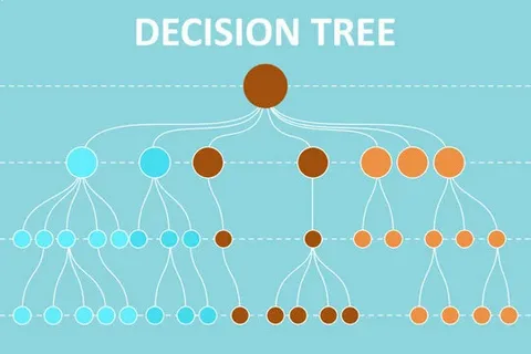
What is a Decision Tree? The Flowchart of Machine Learning

Imagine you’re trying to decide if you should play golf today. Your decision process might look like this:

1. Is it sunny? If no, you stay in. If yes, you proceed.
2. Is it humid? If yes, maybe you reconsider. If no, you proceed.
3. Is it windy? If too windy, you might not go. If it’s calm, you go play.

This step-by-step, question-based process is the exact logic of a Decision Tree. It’s a flowchart-like structure where:

• Internal Node: Represents a “test” on a feature (e.g., “Is it sunny?”).
• Branch: Represents the outcome of the test (e.g., “Yes” or “No”).
• Leaf Node: Represents the final decision or output (e.g., “Play Golf” or “Don’t Play Golf”).

In machine learning, we use data to automatically build this optimal sequence of questions.

How Decision Trees “Learn”: The Splitting Mechanism

The core concept of a Decision Tree is recursive partitioning. It splits the data into subsets based on the value of a feature. The goal is to create subsets that are as “pure” as possible—meaning they contain data points predominantly from a single class.

But how does the algorithm decide which feature to split on, and where? It uses specific criteria to find the most informative split.

1. Gini Impurity

Gini Impurity is a measure of how often a randomly chosen element would be incorrectly labeled if it was randomly labeled according to the distribution of labels in the subset.

• Think of it as: A measure of “chaos” or “disorder.”
• Formula: Gini = 1 - Σ (p_i)² where p_i is the probability of a class in the node.
• A Gini of 0 means perfect purity (all elements are of one class).
• A higher Gini means more impurity.

The algorithm calculates the Gini Impurity for all possible splits and chooses the one that results in the largest reduction in impurity (i.e., the largest “Gini Gain”).

2. Information Gain (using Entropy)

Entropy, borrowed from information theory, measures the amount of uncertainty or randomness.

• Formula: Entropy = - Σ (p_i * log2(p_i))
• Information Gain is the reduction in entropy after a dataset is split. The algorithm seeks the split that provides the highest Information Gain—the one that most reduces uncertainty about the target variable.

Simple Analogy: Imagine a bag of mixed colored balls. A “pure” split would be one action that separates all the red balls into one bag and all the blue balls into another. Gini and Information Gain are different ways of quantifying how good a particular splitting action is.

A Practical Example: Building a Decision Tree Classifier

Let’s use a classic dataset: the Iris flower dataset. Our goal is to classify the species of an iris flower based on its sepal and petal measurements.

Sepal Length	Sepal Width	Petal Length	Petal Width	Species
5.1	3.5	1.4	0.2	Setosa
7.0	3.2	4.7	1.4	Versicolor
6.3	3.3	6.0	2.5	Virginica
…	…	…	…	…

The Decision Tree algorithm will:

1. Start at the root: Look at all features and all possible split points.
2. Find the best split: Calculate Gini Gain/Information Gain for a split on “Petal Length < 2.45 cm” vs. “Petal Width < 1.75 cm”, etc.
3. It might find that the best first question is: “Is Petal Length less than 2.45 cm?”
   • If YES, the flower is almost certainly a Setosa. This branch is now a pure leaf node.
   • If NO, it moves to the next question, perhaps: “Is Petal Width less than 1.75 cm?”
     • If YES, classify as Versicolor.
     • If NO, classify as Virginica.

This creates a clear, interpretable model.

Pros and Cons of Decision Trees

Advantages (The “Pros”)

• Highly Interpretable: The model’s logic is easy to understand and visualize. You can explain a prediction to a non-technical audience.
• Few Data Preprocessing Steps: No need for feature scaling (standardization/normalization) and can handle missing values relatively well.
• Handles Both Numerical and Categorical Data.
• Non-Parametric: Makes no assumptions about the underlying distribution of the data.

Disadvantages (The “Cons”)

• Prone to Overfitting: A tree can keep growing until it memorizes the training data, capturing noise as if it were a pattern. This hurts its performance on new, unseen data. This is their biggest weakness.
• High Variance: Small changes in the training data can result in a completely different tree structure.
• Can Be Biased: If one class is dominant, the tree can become biased.

So, how do we overcome these critical flaws? The answer lies in the power of the crowd.

---

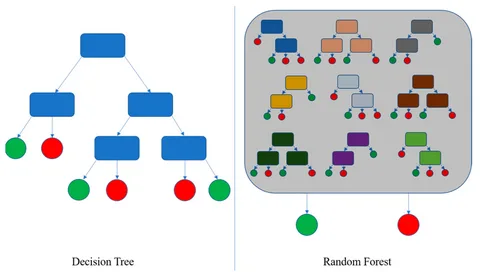
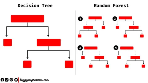
What is a Random Forest? The Wisdom of Crowds

A Random Forest is an ensemble learning method, specifically a Bagging (Bootstrap Aggregating) algorithm. It’s built on a beautifully simple idea:

“Instead of relying on one single, overfitted Decision Tree, why not create hundreds of them and let them vote on the final answer?”

A Random Forest is literally a forest of Decision Trees. The “Random” part comes from two key sources of randomness injected during the training process.

read more about Linear Regression Explained for Beginners: Theory & Python Code

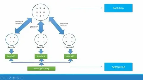
How a Random Forest is Built: The “Bagging” Process

1. Create Multiple Datasets (Bootstrapping): From the original training data, create multiple new datasets by randomly sampling with replacement. This means some data points will be repeated, and others will be left out (these are called “Out-of-Bag” samples).
2. Train a Decision Tree on Each Dataset: For each of these bootstrapped datasets, train a Decision Tree.
   • Key Twist: When splitting a node, instead of considering all features, the algorithm randomly selects a subset of features (e.g., the square root of the total number) to find the best split. This de-correlates the trees, forcing them to learn different aspects of the data.
3. Aggregate the Results:
   • For Classification: Each tree “votes” for a class. The class with the most votes becomes the Random Forest’s prediction.
   • For Regression: The final prediction is the average of the predictions from all the individual trees.

Why Random Forests Are So Powerful

By combining many weak, overfitted learners (individual trees), the Random Forest creates a single strong learner that is:

• Highly Accurate: Consistently performs well across a wide range of problems.
• Robust to Overfitting: The averaging effect of multiple trees cancels out their individual errors and overfitting tendencies.
• Low Variance: Much more stable than a single Decision Tree. Changes in the dataset have a minimal impact on the overall forest.
• Provides Feature Importance: It can measure which features were most influential in making predictions.

Random Forest vs. Decision Tree: A Quick Comparison

Feature	Decision Tree	Random Forest
Interpretability	High (Easy to visualize and explain)	Low (A “black box” compared to a single tree)
Performance	Good, but prone to overfitting	Excellent, state-of-the-art for tabular data
Overfitting	Highly prone	Robust against
Training Speed	Fast	Slower (but can be parallelized)
Prediction Speed	Very Fast	Slower (has to run through many trees)

---

Hands-On Implementation with Python (Scikit-Learn)

Let’s see how easy it is to implement these algorithms using Python’s scikit-learn library.

Step 1: Import Libraries and Load Data

python

# Import necessary libraries
import pandas as pd
from sklearn.model_selection import train_test_split
from sklearn.tree import DecisionTreeClassifier
from sklearn.ensemble import RandomForestClassifier
from sklearn.metrics import accuracy_score
from sklearn.datasets import load_iris

# Load the Iris dataset
iris = load_iris()
X = iris.data  # Features
y = iris.target # Target variable

# Split the data into training and testing sets
X_train, X_test, y_train, y_test = train_test_split(X, y, test_size=0.3, random_state=42)

Step 2: Train a Decision Tree Classifier

python

# Create and train the Decision Tree model
dt_model = DecisionTreeClassifier(random_state=42)
dt_model.fit(X_train, y_train)

# Make predictions on the test set
y_pred_dt = dt_model.predict(X_test)

# Evaluate the model
print(f"Decision Tree Accuracy: {accuracy_score(y_test, y_pred_dt):.2f}")
# Output: Decision Tree Accuracy: 1.00

Step 3: Train a Random Forest Classifier

python

# Create and train the Random Forest model
rf_model = RandomForestClassifier(n_estimators=100, random_state=42) # 100 trees in the forest
rf_model.fit(X_train, y_train)

# Make predictions
y_pred_rf = rf_model.predict(X_test)

# Evaluate the model
print(f"Random Forest Accuracy: {accuracy_score(y_test, y_pred_rf):.2f}")
# Output: Random Forest Accuracy: 1.00

Step 4: Visualizing a Decision Tree

You can visualize the tree to understand its logic (this works best for small trees).

python

from sklearn.tree import plot_tree
import matplotlib.pyplot as plt

plt.figure(figsize=(12,8))
plot_tree(dt_model, feature_names=iris.feature_names, class_names=iris.target_names, filled=True)
plt.show()

Step 5: Analyzing Feature Importance

Random Forests can tell us which features mattered most.

python

# Get feature importances
importances = rf_model.feature_importances_
feature_names = iris.feature_names

# Create a DataFrame for a nice display
feature_imp_df = pd.DataFrame({'Feature': feature_names, 'Importance': importances})
feature_imp_df = feature_imp_df.sort_values('Importance', ascending=False)

print(feature_imp_df)

This might show that petal length and petal width are the most critical features for classifying iris species.

Conclusion: Which One Should You Use?

The choice between a Decision Tree and a Random Forest boils down to the trade-off between interpretability and performance.

• Use a Single Decision Tree when: You need a simple, transparent model for a small dataset, and explaining the “why” behind a prediction is crucial (e.g., loan application decisions, medical diagnosis reasoning).
• Use a Random Forest when: Your primary goal is high predictive accuracy, and you are willing to sacrifice some interpretability. It is the go-to algorithm for many practical, real-world machine learning problems.

By understanding the foundational principles of Decision Trees and the ensemble power of Random Forests, you are now equipped with two of the most versatile tools in the machine learning landscape. Start experimenting with the code, apply it to your own datasets, and witness the power of these remarkable algorithms.